Standardized Total Effect Centrality

Usage

TotalCentralStd(phi, sigma, delta_t, tol = 0.001)

Arguments

phi: Numeric matrix. The drift matrix (\(\boldsymbol{\Phi}\)). phi should have row and column names pertaining to the variables in the system.
sigma: Numeric matrix. The process noise covariance matrix (\(\boldsymbol{\Sigma}\)).
delta_t: Vector of positive numbers. Time interval (\(\Delta t\)).
tol: Numeric. Smallest possible time interval to allow.

Value

Returns an object of class ctmedmed which is a list with the following elements:

call: Function call.
args: Function arguments.
fun: Function used ("TotalCentralStd").
output: A matrix of standardized total effect centrality.

Details

The standardized total effect centrality of a variable is the sum of the standardized total effects of a variable on all other variables at a particular time interval.

Other Continuous-Time Mediation Functions: BootBeta(), BootBetaStd(), BootDirectCentral(), BootIndirectCentral(), BootMed(), BootMedStd(), BootTotalCentral(), DeltaBeta(), DeltaBetaStd(), DeltaDirectCentral(), DeltaIndirectCentral(), DeltaMed(), DeltaMedStd(), DeltaTotalCentral(), Direct(), DirectCentral(), DirectCentralStd(), DirectStd(), Indirect(), IndirectCentral(), IndirectCentralStd(), IndirectStd(), MCBeta(), MCBetaStd(), MCDirectCentral(), MCIndirectCentral(), MCMed(), MCMedStd(), MCPhi(), MCPhiSigma(), MCTotalCentral(), Med(), MedStd(), PosteriorBeta(), PosteriorDirectCentral(), PosteriorIndirectCentral(), PosteriorMed(), PosteriorTotalCentral(), Total(), TotalCentral(), TotalStd(), Trajectory()

Author

Ivan Jacob Agaloos Pesigan

Examples

phi <- matrix(
  data = c(
    -0.357, 0.771, -0.450,
    0.0, -0.511, 0.729,
    0, 0, -0.693
  ),
  nrow = 3
)
colnames(phi) <- rownames(phi) <- c("x", "m", "y")
sigma <- matrix(
  data = c(
    0.24455556, 0.02201587, -0.05004762,
    0.02201587, 0.07067800, 0.01539456,
    -0.05004762, 0.01539456, 0.07553061
  ),
  nrow = 3
)

# Specific time interval ----------------------------------------------------
TotalCentralStd(
  phi = phi,
  sigma = sigma,
  delta_t = 1
)
#> Call:
#> TotalCentralStd(phi = phi, sigma = sigma, delta_t = 1)
#> 
#> Total Effect Centrality
#>      interval      x      m y
#> [1,]        1 0.2819 0.5494 0

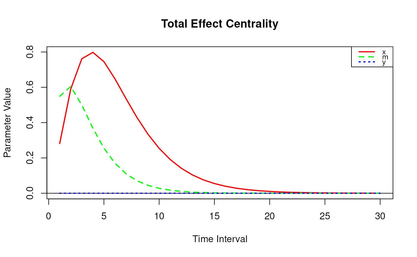
# Range of time intervals ---------------------------------------------------
total_central_std <- TotalCentralStd(
  phi = phi,
  sigma = sigma,
  delta_t = 1:30
)
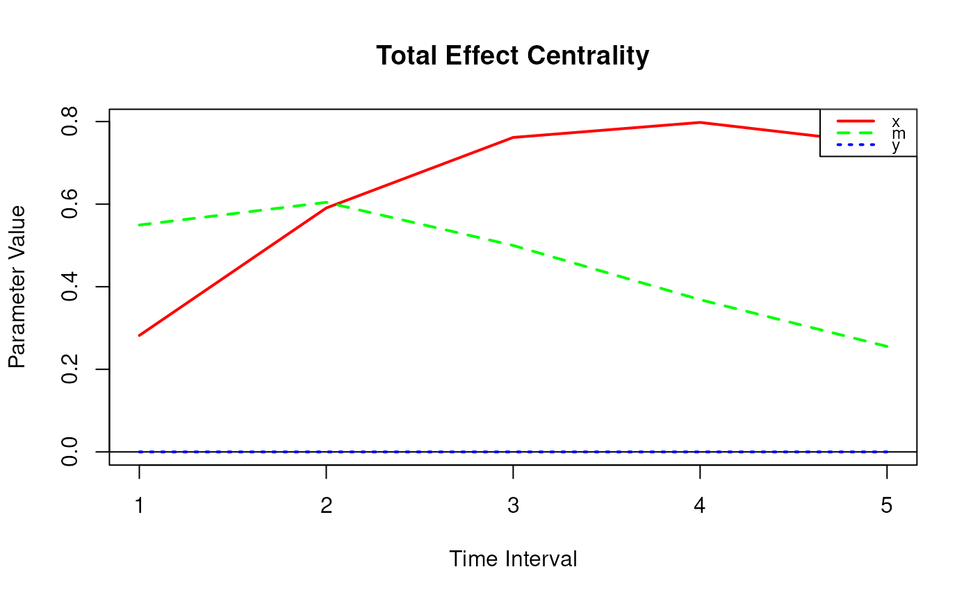
plot(total_central_std)


# Methods -------------------------------------------------------------------
# TotalCentralStd has a number of methods including
# print, summary, and plot
total_central_std <- TotalCentralStd(
  phi = phi,
  sigma = sigma,
  delta_t = 1:5
)
print(total_central_std)
#> Call:
#> TotalCentralStd(phi = phi, sigma = sigma, delta_t = 1:5)
#> 
#> Total Effect Centrality
#>      interval      x      m y
#> [1,]        1 0.2819 0.5494 0
#> [2,]        2 0.5907 0.6044 0
#> [3,]        3 0.7616 0.4999 0
#> [4,]        4 0.7979 0.3686 0
#> [5,]        5 0.7453 0.2555 0
summary(total_central_std)
#> Call:
#> TotalCentralStd(phi = phi, sigma = sigma, delta_t = 1:5)
#> 
#> Total Effect Centrality
#>      interval      x      m y
#> [1,]        1 0.2819 0.5494 0
#> [2,]        2 0.5907 0.6044 0
#> [3,]        3 0.7616 0.4999 0
#> [4,]        4 0.7979 0.3686 0
#> [5,]        5 0.7453 0.2555 0
plot(total_central_std)