Delta Method Sampling Variance-Covariance Matrix for the Total, Direct, and Indirect Effects of X on Y Through M Over a Specific Time Interval or a Range of Time Intervals
Source:R/cTMed-delta-med.R
DeltaMed.RdThis function computes the delta method sampling variance-covariance matrix for the total, direct, and indirect effects of the independent variable \(X\) on the dependent variable \(Y\) through mediator variables \(\mathbf{m}\) over a specific time interval \(\Delta t\) or a range of time intervals using the first-order stochastic differential equation model's drift matrix \(\boldsymbol{\Phi}\).
Arguments
- phi
Numeric matrix. The drift matrix (\(\boldsymbol{\Phi}\)).
phishould have row and column names pertaining to the variables in the system.- vcov_phi_vec
Numeric matrix. The sampling variance-covariance matrix of \(\mathrm{vec} \left( \boldsymbol{\Phi} \right)\).
- delta_t
Vector of positive numbers. Time interval (\(\Delta t\)).
- from
Character string. Name of the independent variable \(X\) in
phi.- to
Character string. Name of the dependent variable \(Y\) in
phi.- med
Character vector. Name/s of the mediator variable/s in
phi.- ncores
Positive integer. Number of cores to use. If
ncores = NULL, use a single core. Consider using multiple cores when the length ofdelta_tis long.- tol
Numeric. Smallest possible time interval to allow.
Value
Returns an object
of class ctmeddelta which is a list with the following elements:
- call
Function call.
- args
Function arguments.
- fun
Function used ("DeltaMed").
- output
A list of length
length(delta_t).
Each element in the output list has the following elements:
- delta_t
Time interval.
- jacobian
Jacobian matrix.
- est
Estimated total, direct, and indirect effects.
- vcov
Sampling variance-covariance matrix of the estimated total, direct, and indirect effects.
Details
See Total(),
Direct(), and
Indirect() for more details.
Delta Method
Let \(\boldsymbol{\theta}\) be \(\mathrm{vec} \left( \boldsymbol{\Phi} \right)\), that is, the elements of the \(\boldsymbol{\Phi}\) matrix in vector form sorted column-wise. Let \(\hat{\boldsymbol{\theta}}\) be \(\mathrm{vec} \left( \hat{\boldsymbol{\Phi}} \right)\). By the multivariate central limit theory, the function \(\mathbf{g}\) using \(\hat{\boldsymbol{\theta}}\) as input can be expressed as:
$$ \sqrt{n} \left( \mathbf{g} \left( \hat{\boldsymbol{\theta}} \right) - \mathbf{g} \left( \boldsymbol{\theta} \right) \right) \xrightarrow[]{ \mathrm{D} } \mathcal{N} \left( 0, \mathbf{J} \boldsymbol{\Gamma} \mathbf{J}^{\prime} \right) $$
where \(\mathbf{J}\) is the matrix of first-order derivatives of the function \(\mathbf{g}\) with respect to the elements of \(\boldsymbol{\theta}\) and \(\boldsymbol{\Gamma}\) is the asymptotic variance-covariance matrix of \(\hat{\boldsymbol{\theta}}\).
From the former, we can derive the distribution of \(\mathbf{g} \left( \hat{\boldsymbol{\theta}} \right)\) as follows:
$$ \mathbf{g} \left( \hat{\boldsymbol{\theta}} \right) \approx \mathcal{N} \left( \mathbf{g} \left( \boldsymbol{\theta} \right) , n^{-1} \mathbf{J} \boldsymbol{\Gamma} \mathbf{J}^{\prime} \right) $$
The uncertainty associated with the estimator \(\mathbf{g} \left( \hat{\boldsymbol{\theta}} \right)\) is, therefore, given by \(n^{-1} \mathbf{J} \boldsymbol{\Gamma} \mathbf{J}^{\prime}\) . When \(\boldsymbol{\Gamma}\) is unknown, by substitution, we can use the estimated sampling variance-covariance matrix of \(\hat{\boldsymbol{\theta}}\), that is, \(\hat{\mathbb{V}} \left( \hat{\boldsymbol{\theta}} \right)\) for \(n^{-1} \boldsymbol{\Gamma}\). Therefore, the sampling variance-covariance matrix of \(\mathbf{g} \left( \hat{\boldsymbol{\theta}} \right)\) is given by
$$ \mathbf{g} \left( \hat{\boldsymbol{\theta}} \right) \approx \mathcal{N} \left( \mathbf{g} \left( \boldsymbol{\theta} \right) , \mathbf{J} \hat{\mathbb{V}} \left( \hat{\boldsymbol{\theta}} \right) \mathbf{J}^{\prime} \right) . $$
References
Bollen, K. A. (1987). Total, direct, and indirect effects in structural equation models. Sociological Methodology, 17, 37. doi:10.2307/271028
Deboeck, P. R., & Preacher, K. J. (2015). No need to be discrete: A method for continuous time mediation analysis. Structural Equation Modeling: A Multidisciplinary Journal, 23 (1), 61-75. doi:10.1080/10705511.2014.973960
Pesigan, I. J. A., Russell, M. A., & Chow, S.-M. (2025). Inferences and effect sizes for direct, indirect, and total effects in continuous-time mediation models. Psychological Methods. doi:10.1037/met0000779
Ryan, O., & Hamaker, E. L. (2021). Time to intervene: A continuous-time approach to network analysis and centrality. Psychometrika, 87 (1), 214-252. doi:10.1007/s11336-021-09767-0
See also
Other Continuous-Time Mediation Functions:
BootBeta(),
BootBetaStd(),
BootDirectCentral(),
BootDirectCentralStd(),
BootIndirectCentral(),
BootIndirectCentralStd(),
BootMed(),
BootMedStd(),
BootTotalCentral(),
BootTotalCentralStd(),
DeltaBeta(),
DeltaBetaStd(),
DeltaDirectCentral(),
DeltaDirectCentralStd(),
DeltaIndirectCentral(),
DeltaMedStd(),
DeltaTotalCentral(),
DeltaTotalCentralStd(),
Direct(),
DirectCentral(),
DirectCentralStd(),
DirectStd(),
Indirect(),
IndirectCentral(),
IndirectCentralStd(),
IndirectStd(),
MCBeta(),
MCBetaStd(),
MCDirectCentral(),
MCDirectCentralStd(),
MCIndirectCentral(),
MCIndirectCentralStd(),
MCMed(),
MCMedStd(),
MCPhi(),
MCPhiSigma(),
MCTotalCentral(),
MCTotalCentralStd(),
Med(),
MedStd(),
PosteriorBeta(),
PosteriorBetaStd(),
PosteriorDirectCentral(),
PosteriorDirectCentralStd(),
PosteriorIndirectCentral(),
PosteriorIndirectCentralStd(),
PosteriorMed(),
PosteriorMedStd(),
PosteriorTotalCentral(),
PosteriorTotalCentralStd(),
Total(),
TotalCentral(),
TotalCentralStd(),
TotalStd(),
Trajectory()
Examples
phi <- matrix(
data = c(
-0.357, 0.771, -0.450,
0.0, -0.511, 0.729,
0, 0, -0.693
),
nrow = 3
)
colnames(phi) <- rownames(phi) <- c("x", "m", "y")
vcov_phi_vec <- matrix(
data = c(
0.00843, 0.00040, -0.00151,
-0.00600, -0.00033, 0.00110,
0.00324, 0.00020, -0.00061,
0.00040, 0.00374, 0.00016,
-0.00022, -0.00273, -0.00016,
0.00009, 0.00150, 0.00012,
-0.00151, 0.00016, 0.00389,
0.00103, -0.00007, -0.00283,
-0.00050, 0.00000, 0.00156,
-0.00600, -0.00022, 0.00103,
0.00644, 0.00031, -0.00119,
-0.00374, -0.00021, 0.00070,
-0.00033, -0.00273, -0.00007,
0.00031, 0.00287, 0.00013,
-0.00014, -0.00170, -0.00012,
0.00110, -0.00016, -0.00283,
-0.00119, 0.00013, 0.00297,
0.00063, -0.00004, -0.00177,
0.00324, 0.00009, -0.00050,
-0.00374, -0.00014, 0.00063,
0.00495, 0.00024, -0.00093,
0.00020, 0.00150, 0.00000,
-0.00021, -0.00170, -0.00004,
0.00024, 0.00214, 0.00012,
-0.00061, 0.00012, 0.00156,
0.00070, -0.00012, -0.00177,
-0.00093, 0.00012, 0.00223
),
nrow = 9
)
# Specific time interval ----------------------------------------------------
DeltaMed(
phi = phi,
vcov_phi_vec = vcov_phi_vec,
delta_t = 1,
from = "x",
to = "y",
med = "m"
)
#> Call:
#> DeltaMed(phi = phi, vcov_phi_vec = vcov_phi_vec, delta_t = 1,
#> from = "x", to = "y", med = "m")
#>
#> Total, Direct, and Indirect Effects
#>
#> effect interval est se z p 2.5% 97.5%
#> 1 total 1 -0.1000 0.0306 -3.2703 0.0011 -0.1600 -0.0401
#> 2 direct 1 -0.2675 0.0394 -6.7894 0.0000 -0.3447 -0.1902
#> 3 indirect 1 0.1674 0.0175 9.5524 0.0000 0.1331 0.2018
# Range of time intervals ---------------------------------------------------
delta <- DeltaMed(
phi = phi,
vcov_phi_vec = vcov_phi_vec,
delta_t = 1:5,
from = "x",
to = "y",
med = "m"
)
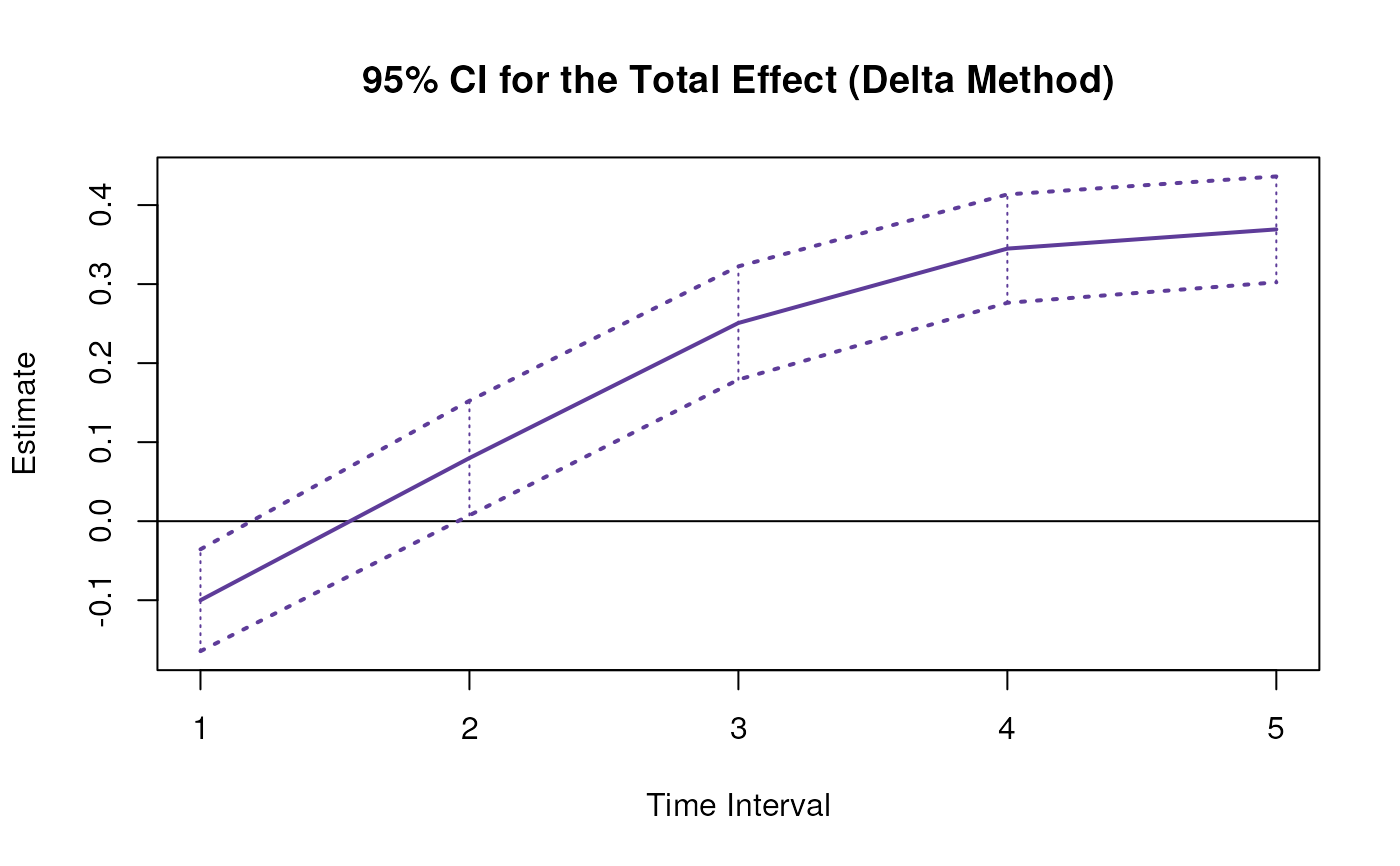
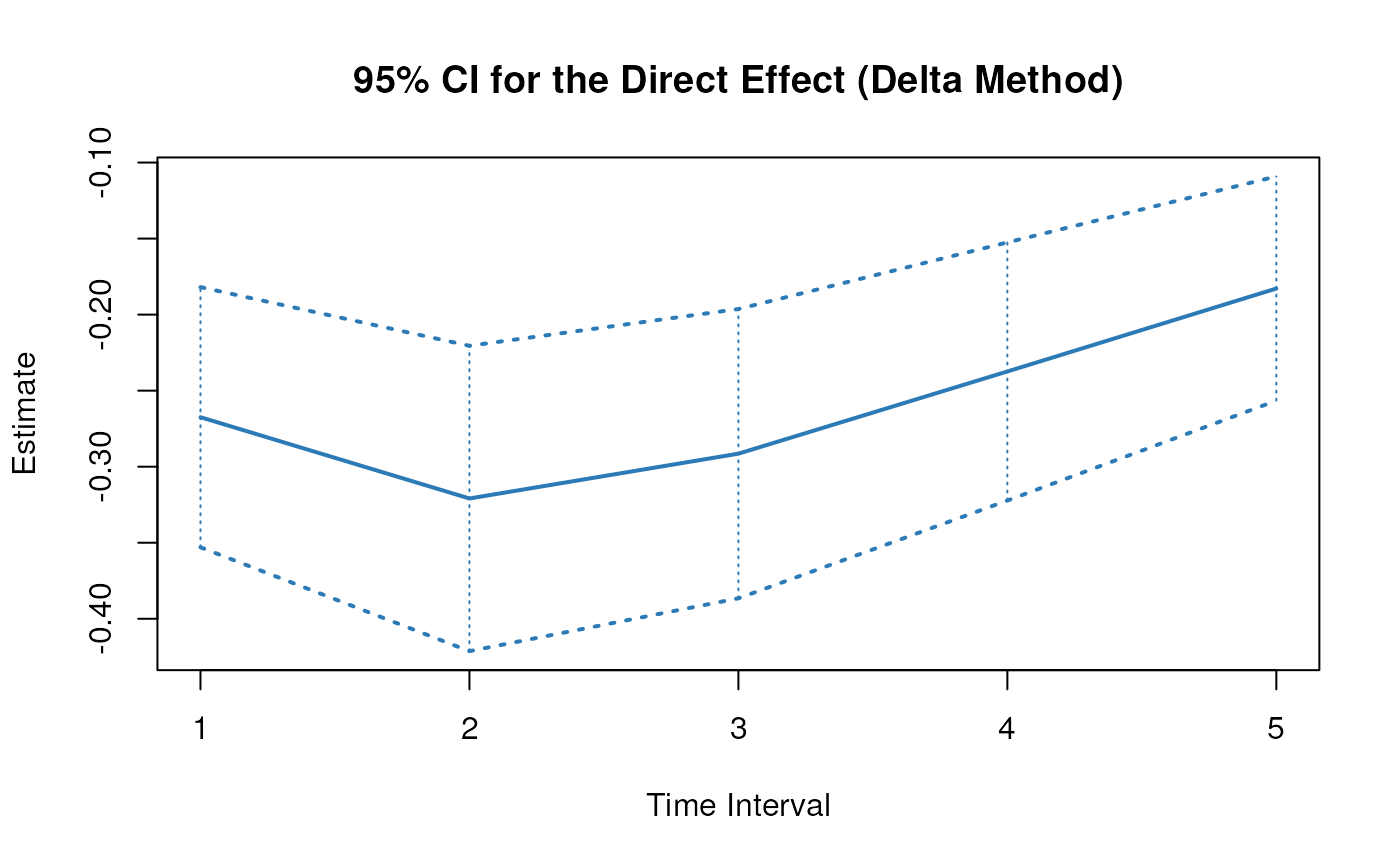
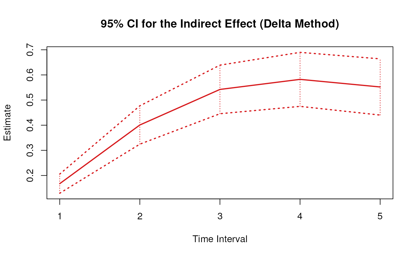
plot(delta)

 # Methods -------------------------------------------------------------------
# DeltaMed has a number of methods including
# print, summary, confint, and plot
print(delta)
#> Call:
#> DeltaMed(phi = phi, vcov_phi_vec = vcov_phi_vec, delta_t = 1:5,
#> from = "x", to = "y", med = "m")
#>
#> Total, Direct, and Indirect Effects
#>
#> effect interval est se z p 2.5% 97.5%
#> 1 total 1 -0.1000 0.0306 -3.2703 0.0011 -0.1600 -0.0401
#> 2 direct 1 -0.2675 0.0394 -6.7894 0.0000 -0.3447 -0.1902
#> 3 indirect 1 0.1674 0.0175 9.5524 0.0000 0.1331 0.2018
#> 4 total 2 0.0799 0.0342 2.3337 0.0196 0.0128 0.1470
#> 5 direct 2 -0.3209 0.0552 -5.8129 0.0000 -0.4291 -0.2127
#> 6 indirect 2 0.4008 0.0461 8.7033 0.0000 0.3105 0.4911
#> 7 total 3 0.2508 0.0353 7.1106 0.0000 0.1817 0.3199
#> 8 direct 3 -0.2914 0.0608 -4.7907 0.0000 -0.4107 -0.1722
#> 9 indirect 3 0.5423 0.0703 7.7121 0.0000 0.4044 0.6801
#> 10 total 4 0.3449 0.0394 8.7512 0.0000 0.2677 0.4222
#> 11 direct 4 -0.2374 0.0604 -3.9333 0.0001 -0.3557 -0.1191
#> 12 indirect 4 0.5823 0.0850 6.8529 0.0000 0.4158 0.7489
#> 13 total 5 0.3693 0.0441 8.3649 0.0000 0.2827 0.4558
#> 14 direct 5 -0.1828 0.0561 -3.2606 0.0011 -0.2928 -0.0729
#> 15 indirect 5 0.5521 0.0899 6.1417 0.0000 0.3759 0.7283
summary(delta)
#> Call:
#> DeltaMed(phi = phi, vcov_phi_vec = vcov_phi_vec, delta_t = 1:5,
#> from = "x", to = "y", med = "m")
#>
#> Total, Direct, and Indirect Effects
#>
#> effect interval est se z p 2.5% 97.5%
#> 1 total 1 -0.1000 0.0306 -3.2703 0.0011 -0.1600 -0.0401
#> 2 direct 1 -0.2675 0.0394 -6.7894 0.0000 -0.3447 -0.1902
#> 3 indirect 1 0.1674 0.0175 9.5524 0.0000 0.1331 0.2018
#> 4 total 2 0.0799 0.0342 2.3337 0.0196 0.0128 0.1470
#> 5 direct 2 -0.3209 0.0552 -5.8129 0.0000 -0.4291 -0.2127
#> 6 indirect 2 0.4008 0.0461 8.7033 0.0000 0.3105 0.4911
#> 7 total 3 0.2508 0.0353 7.1106 0.0000 0.1817 0.3199
#> 8 direct 3 -0.2914 0.0608 -4.7907 0.0000 -0.4107 -0.1722
#> 9 indirect 3 0.5423 0.0703 7.7121 0.0000 0.4044 0.6801
#> 10 total 4 0.3449 0.0394 8.7512 0.0000 0.2677 0.4222
#> 11 direct 4 -0.2374 0.0604 -3.9333 0.0001 -0.3557 -0.1191
#> 12 indirect 4 0.5823 0.0850 6.8529 0.0000 0.4158 0.7489
#> 13 total 5 0.3693 0.0441 8.3649 0.0000 0.2827 0.4558
#> 14 direct 5 -0.1828 0.0561 -3.2606 0.0011 -0.2928 -0.0729
#> 15 indirect 5 0.5521 0.0899 6.1417 0.0000 0.3759 0.7283
confint(delta, level = 0.95)
#> effect interval 2.5 % 97.5 %
#> 1 total 1 -0.15999452 -0.04008223
#> 2 direct 1 -0.34466208 -0.19024569
#> 3 indirect 1 0.13306530 0.20176572
#> 4 total 2 0.01279611 0.14700550
#> 5 direct 2 -0.42910491 -0.21270209
#> 6 indirect 2 0.31054364 0.49106497
#> 7 total 3 0.18167990 0.31994775
#> 8 direct 3 -0.41067673 -0.17220847
#> 9 indirect 3 0.40444738 0.68006547
#> 10 total 4 0.26767567 0.42218015
#> 11 direct 4 -0.35568031 -0.11909972
#> 12 indirect 4 0.41577174 0.74886411
#> 13 total 5 0.28273472 0.45577286
#> 14 direct 5 -0.29275471 -0.07293472
#> 15 indirect 5 0.37591173 0.72828528
plot(delta)
# Methods -------------------------------------------------------------------
# DeltaMed has a number of methods including
# print, summary, confint, and plot
print(delta)
#> Call:
#> DeltaMed(phi = phi, vcov_phi_vec = vcov_phi_vec, delta_t = 1:5,
#> from = "x", to = "y", med = "m")
#>
#> Total, Direct, and Indirect Effects
#>
#> effect interval est se z p 2.5% 97.5%
#> 1 total 1 -0.1000 0.0306 -3.2703 0.0011 -0.1600 -0.0401
#> 2 direct 1 -0.2675 0.0394 -6.7894 0.0000 -0.3447 -0.1902
#> 3 indirect 1 0.1674 0.0175 9.5524 0.0000 0.1331 0.2018
#> 4 total 2 0.0799 0.0342 2.3337 0.0196 0.0128 0.1470
#> 5 direct 2 -0.3209 0.0552 -5.8129 0.0000 -0.4291 -0.2127
#> 6 indirect 2 0.4008 0.0461 8.7033 0.0000 0.3105 0.4911
#> 7 total 3 0.2508 0.0353 7.1106 0.0000 0.1817 0.3199
#> 8 direct 3 -0.2914 0.0608 -4.7907 0.0000 -0.4107 -0.1722
#> 9 indirect 3 0.5423 0.0703 7.7121 0.0000 0.4044 0.6801
#> 10 total 4 0.3449 0.0394 8.7512 0.0000 0.2677 0.4222
#> 11 direct 4 -0.2374 0.0604 -3.9333 0.0001 -0.3557 -0.1191
#> 12 indirect 4 0.5823 0.0850 6.8529 0.0000 0.4158 0.7489
#> 13 total 5 0.3693 0.0441 8.3649 0.0000 0.2827 0.4558
#> 14 direct 5 -0.1828 0.0561 -3.2606 0.0011 -0.2928 -0.0729
#> 15 indirect 5 0.5521 0.0899 6.1417 0.0000 0.3759 0.7283
summary(delta)
#> Call:
#> DeltaMed(phi = phi, vcov_phi_vec = vcov_phi_vec, delta_t = 1:5,
#> from = "x", to = "y", med = "m")
#>
#> Total, Direct, and Indirect Effects
#>
#> effect interval est se z p 2.5% 97.5%
#> 1 total 1 -0.1000 0.0306 -3.2703 0.0011 -0.1600 -0.0401
#> 2 direct 1 -0.2675 0.0394 -6.7894 0.0000 -0.3447 -0.1902
#> 3 indirect 1 0.1674 0.0175 9.5524 0.0000 0.1331 0.2018
#> 4 total 2 0.0799 0.0342 2.3337 0.0196 0.0128 0.1470
#> 5 direct 2 -0.3209 0.0552 -5.8129 0.0000 -0.4291 -0.2127
#> 6 indirect 2 0.4008 0.0461 8.7033 0.0000 0.3105 0.4911
#> 7 total 3 0.2508 0.0353 7.1106 0.0000 0.1817 0.3199
#> 8 direct 3 -0.2914 0.0608 -4.7907 0.0000 -0.4107 -0.1722
#> 9 indirect 3 0.5423 0.0703 7.7121 0.0000 0.4044 0.6801
#> 10 total 4 0.3449 0.0394 8.7512 0.0000 0.2677 0.4222
#> 11 direct 4 -0.2374 0.0604 -3.9333 0.0001 -0.3557 -0.1191
#> 12 indirect 4 0.5823 0.0850 6.8529 0.0000 0.4158 0.7489
#> 13 total 5 0.3693 0.0441 8.3649 0.0000 0.2827 0.4558
#> 14 direct 5 -0.1828 0.0561 -3.2606 0.0011 -0.2928 -0.0729
#> 15 indirect 5 0.5521 0.0899 6.1417 0.0000 0.3759 0.7283
confint(delta, level = 0.95)
#> effect interval 2.5 % 97.5 %
#> 1 total 1 -0.15999452 -0.04008223
#> 2 direct 1 -0.34466208 -0.19024569
#> 3 indirect 1 0.13306530 0.20176572
#> 4 total 2 0.01279611 0.14700550
#> 5 direct 2 -0.42910491 -0.21270209
#> 6 indirect 2 0.31054364 0.49106497
#> 7 total 3 0.18167990 0.31994775
#> 8 direct 3 -0.41067673 -0.17220847
#> 9 indirect 3 0.40444738 0.68006547
#> 10 total 4 0.26767567 0.42218015
#> 11 direct 4 -0.35568031 -0.11909972
#> 12 indirect 4 0.41577174 0.74886411
#> 13 total 5 0.28273472 0.45577286
#> 14 direct 5 -0.29275471 -0.07293472
#> 15 indirect 5 0.37591173 0.72828528
plot(delta)