Delta Method Sampling Variance-Covariance Matrix for the Elements of the Matrix of Lagged Coefficients Over a Specific Time Interval or a Range of Time Intervals
Source:R/cTMed-delta-beta.R
DeltaBeta.RdThis function computes the delta method sampling variance-covariance matrix for the elements of the matrix of lagged coefficients \(\boldsymbol{\beta}\) over a specific time interval \(\Delta t\) or a range of time intervals using the first-order stochastic differential equation model's drift matrix \(\boldsymbol{\Phi}\).
Arguments
- phi
Numeric matrix. The drift matrix (\(\boldsymbol{\Phi}\)).
phishould have row and column names pertaining to the variables in the system.- vcov_phi_vec
Numeric matrix. The sampling variance-covariance matrix of \(\mathrm{vec} \left( \boldsymbol{\Phi} \right)\).
- delta_t
Vector of positive numbers. Time interval (\(\Delta t\)).
- ncores
Positive integer. Number of cores to use. If
ncores = NULL, use a single core. Consider using multiple cores when the length ofdelta_tis long.- tol
Numeric. Smallest possible time interval to allow.
Value
Returns an object
of class ctmeddelta which is a list with the following elements:
- call
Function call.
- args
Function arguments.
- fun
Function used ("DeltaBeta").
- output
A list of length
length(delta_t).
Each element in the output list has the following elements:
- delta_t
Time interval.
- jacobian
Jacobian matrix.
- est
Estimated elements of the matrix of lagged coefficients.
- vcov
Sampling variance-covariance matrix of estimated elements of the matrix of lagged coefficients.
Details
See Total().
Delta Method
Let \(\boldsymbol{\theta}\) be \(\mathrm{vec} \left( \boldsymbol{\Phi} \right)\), that is, the elements of the \(\boldsymbol{\Phi}\) matrix in vector form sorted column-wise. Let \(\hat{\boldsymbol{\theta}}\) be \(\mathrm{vec} \left( \hat{\boldsymbol{\Phi}} \right)\). By the multivariate central limit theory, the function \(\mathbf{g}\) using \(\hat{\boldsymbol{\theta}}\) as input can be expressed as:
$$ \sqrt{n} \left( \mathbf{g} \left( \hat{\boldsymbol{\theta}} \right) - \mathbf{g} \left( \boldsymbol{\theta} \right) \right) \xrightarrow[]{ \mathrm{D} } \mathcal{N} \left( 0, \mathbf{J} \boldsymbol{\Gamma} \mathbf{J}^{\prime} \right) $$
where \(\mathbf{J}\) is the matrix of first-order derivatives of the function \(\mathbf{g}\) with respect to the elements of \(\boldsymbol{\theta}\) and \(\boldsymbol{\Gamma}\) is the asymptotic variance-covariance matrix of \(\hat{\boldsymbol{\theta}}\).
From the former, we can derive the distribution of \(\mathbf{g} \left( \hat{\boldsymbol{\theta}} \right)\) as follows:
$$ \mathbf{g} \left( \hat{\boldsymbol{\theta}} \right) \approx \mathcal{N} \left( \mathbf{g} \left( \boldsymbol{\theta} \right) , n^{-1} \mathbf{J} \boldsymbol{\Gamma} \mathbf{J}^{\prime} \right) $$
The uncertainty associated with the estimator \(\mathbf{g} \left( \hat{\boldsymbol{\theta}} \right)\) is, therefore, given by \(n^{-1} \mathbf{J} \boldsymbol{\Gamma} \mathbf{J}^{\prime}\) . When \(\boldsymbol{\Gamma}\) is unknown, by substitution, we can use the estimated sampling variance-covariance matrix of \(\hat{\boldsymbol{\theta}}\), that is, \(\hat{\mathbb{V}} \left( \hat{\boldsymbol{\theta}} \right)\) for \(n^{-1} \boldsymbol{\Gamma}\). Therefore, the sampling variance-covariance matrix of \(\mathbf{g} \left( \hat{\boldsymbol{\theta}} \right)\) is given by
$$ \mathbf{g} \left( \hat{\boldsymbol{\theta}} \right) \approx \mathcal{N} \left( \mathbf{g} \left( \boldsymbol{\theta} \right) , \mathbf{J} \hat{\mathbb{V}} \left( \hat{\boldsymbol{\theta}} \right) \mathbf{J}^{\prime} \right) . $$
References
Bollen, K. A. (1987). Total, direct, and indirect effects in structural equation models. Sociological Methodology, 17, 37. doi:10.2307/271028
Deboeck, P. R., & Preacher, K. J. (2015). No need to be discrete: A method for continuous time mediation analysis. Structural Equation Modeling: A Multidisciplinary Journal, 23 (1), 61-75. doi:10.1080/10705511.2014.973960
Pesigan, I. J. A., Russell, M. A., & Chow, S.-M. (2025). Inferences and effect sizes for direct, indirect, and total effects in continuous-time mediation models. Psychological Methods. doi:10.1037/met0000779
Ryan, O., & Hamaker, E. L. (2021). Time to intervene: A continuous-time approach to network analysis and centrality. Psychometrika, 87 (1), 214-252. doi:10.1007/s11336-021-09767-0
See also
Other Continuous-Time Mediation Functions:
BootBeta(),
BootBetaStd(),
BootDirectCentral(),
BootDirectCentralStd(),
BootIndirectCentral(),
BootIndirectCentralStd(),
BootMed(),
BootMedStd(),
BootTotalCentral(),
BootTotalCentralStd(),
DeltaBetaStd(),
DeltaDirectCentral(),
DeltaDirectCentralStd(),
DeltaIndirectCentral(),
DeltaMed(),
DeltaMedStd(),
DeltaTotalCentral(),
DeltaTotalCentralStd(),
Direct(),
DirectCentral(),
DirectCentralStd(),
DirectStd(),
Indirect(),
IndirectCentral(),
IndirectCentralStd(),
IndirectStd(),
MCBeta(),
MCBetaStd(),
MCDirectCentral(),
MCDirectCentralStd(),
MCIndirectCentral(),
MCIndirectCentralStd(),
MCMed(),
MCMedStd(),
MCPhi(),
MCPhiSigma(),
MCTotalCentral(),
MCTotalCentralStd(),
Med(),
MedStd(),
PosteriorBeta(),
PosteriorBetaStd(),
PosteriorDirectCentral(),
PosteriorDirectCentralStd(),
PosteriorIndirectCentral(),
PosteriorIndirectCentralStd(),
PosteriorMed(),
PosteriorMedStd(),
PosteriorTotalCentral(),
PosteriorTotalCentralStd(),
Total(),
TotalCentral(),
TotalCentralStd(),
TotalStd(),
Trajectory()
Examples
phi <- matrix(
data = c(
-0.357, 0.771, -0.450,
0.0, -0.511, 0.729,
0, 0, -0.693
),
nrow = 3
)
colnames(phi) <- rownames(phi) <- c("x", "m", "y")
vcov_phi_vec <- matrix(
data = c(
0.00843, 0.00040, -0.00151,
-0.00600, -0.00033, 0.00110,
0.00324, 0.00020, -0.00061,
0.00040, 0.00374, 0.00016,
-0.00022, -0.00273, -0.00016,
0.00009, 0.00150, 0.00012,
-0.00151, 0.00016, 0.00389,
0.00103, -0.00007, -0.00283,
-0.00050, 0.00000, 0.00156,
-0.00600, -0.00022, 0.00103,
0.00644, 0.00031, -0.00119,
-0.00374, -0.00021, 0.00070,
-0.00033, -0.00273, -0.00007,
0.00031, 0.00287, 0.00013,
-0.00014, -0.00170, -0.00012,
0.00110, -0.00016, -0.00283,
-0.00119, 0.00013, 0.00297,
0.00063, -0.00004, -0.00177,
0.00324, 0.00009, -0.00050,
-0.00374, -0.00014, 0.00063,
0.00495, 0.00024, -0.00093,
0.00020, 0.00150, 0.00000,
-0.00021, -0.00170, -0.00004,
0.00024, 0.00214, 0.00012,
-0.00061, 0.00012, 0.00156,
0.00070, -0.00012, -0.00177,
-0.00093, 0.00012, 0.00223
),
nrow = 9
)
# Specific time interval ----------------------------------------------------
DeltaBeta(
phi = phi,
vcov_phi_vec = vcov_phi_vec,
delta_t = 1
)
#> Call:
#> DeltaBeta(phi = phi, vcov_phi_vec = vcov_phi_vec, delta_t = 1)
#>
#> Elements of the matrix of lagged coefficients
#>
#> effect interval est se z p 2.5% 97.5%
#> 1 from x to x 1 0.6998 0.0471 14.8688 0.0000 0.6075 0.7920
#> 2 from x to m 1 0.5000 0.0352 14.1965 0.0000 0.4310 0.5691
#> 3 from x to y 1 -0.1000 0.0306 -3.2703 0.0011 -0.1600 -0.0401
#> 4 from m to x 1 0.0000 0.0435 0.0000 1.0000 -0.0852 0.0852
#> 5 from m to m 1 0.5999 0.0326 18.3826 0.0000 0.5359 0.6639
#> 6 from m to y 1 0.3998 0.0284 14.0593 0.0000 0.3441 0.4556
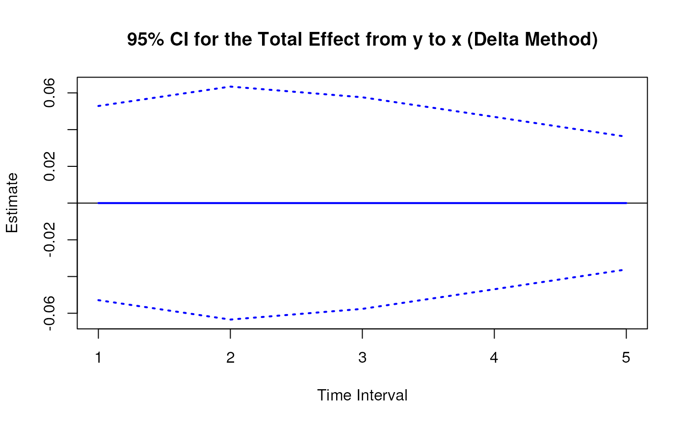
#> 7 from y to x 1 0.0000 0.0418 0.0000 1.0000 -0.0820 0.0820
#> 8 from y to m 1 0.0000 0.0311 0.0000 1.0000 -0.0609 0.0609
#> 9 from y to y 1 0.5001 0.0274 18.2776 0.0000 0.4464 0.5537
# Range of time intervals ---------------------------------------------------
delta <- DeltaBeta(
phi = phi,
vcov_phi_vec = vcov_phi_vec,
delta_t = 1:5
)
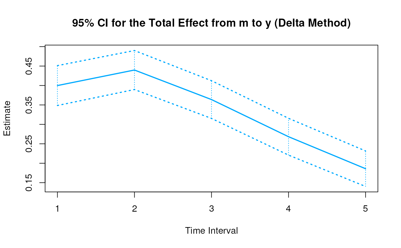
plot(delta)


 # Methods -------------------------------------------------------------------
# DeltaBeta has a number of methods including
# print, summary, confint, and plot
print(delta)
#> Call:
#> DeltaBeta(phi = phi, vcov_phi_vec = vcov_phi_vec, delta_t = 1:5)
#>
#> Elements of the matrix of lagged coefficients
#>
#> effect interval est se z p 2.5% 97.5%
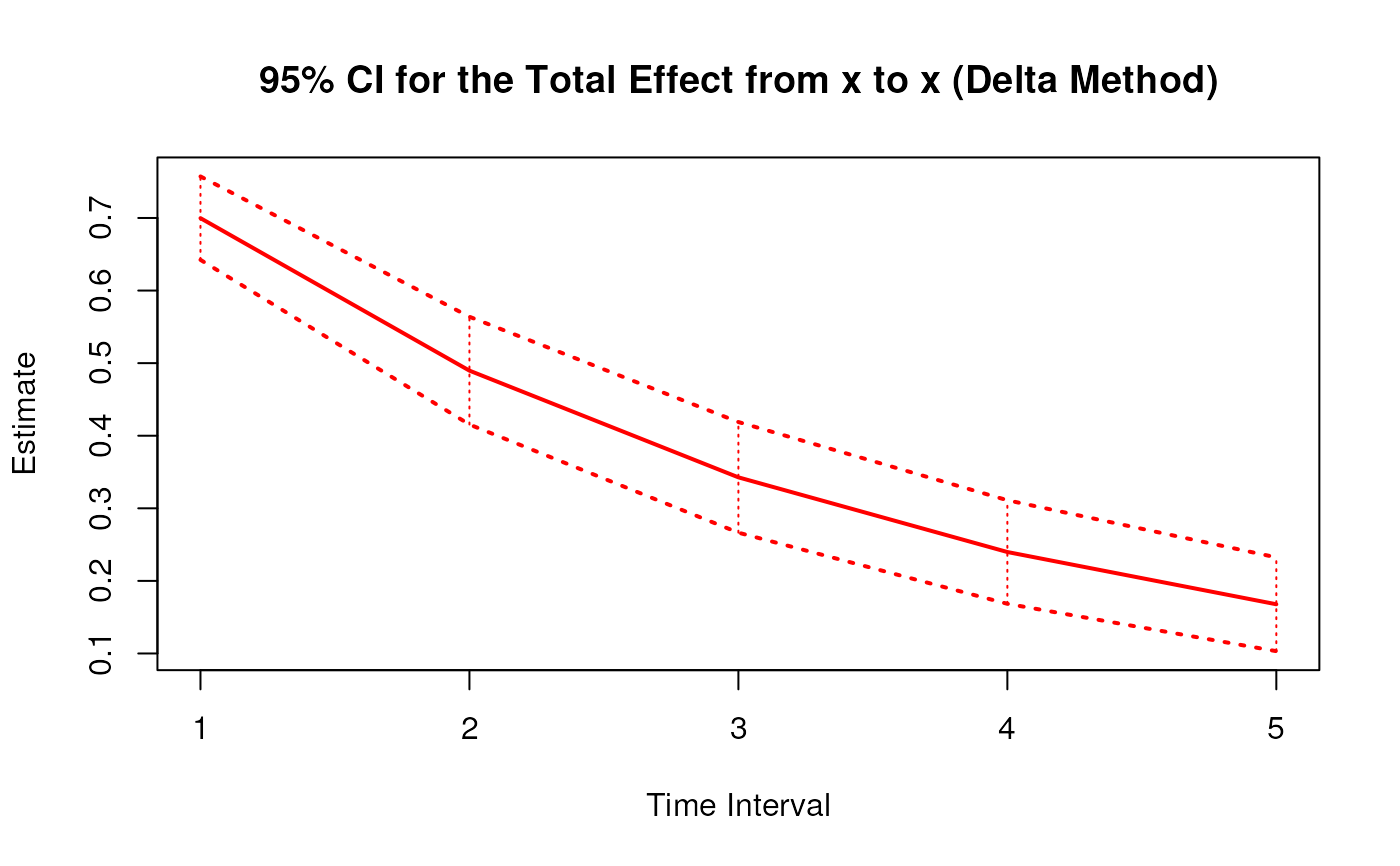
#> 1 from x to x 1 0.6998 0.0471 14.8688 0.0000 0.6075 0.7920
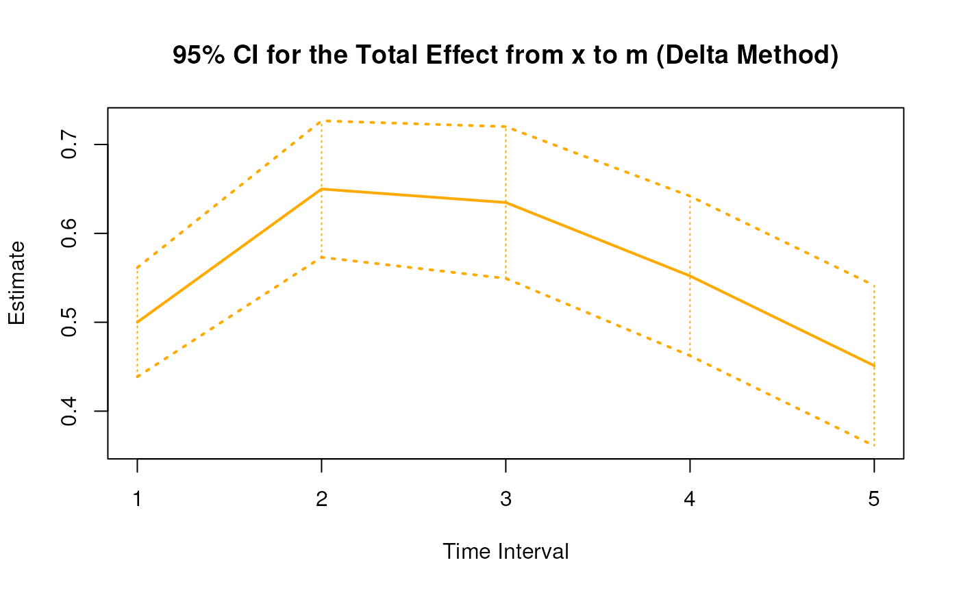
#> 2 from x to m 1 0.5000 0.0352 14.1965 0.0000 0.4310 0.5691
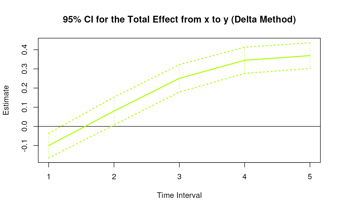
#> 3 from x to y 1 -0.1000 0.0306 -3.2703 0.0011 -0.1600 -0.0401
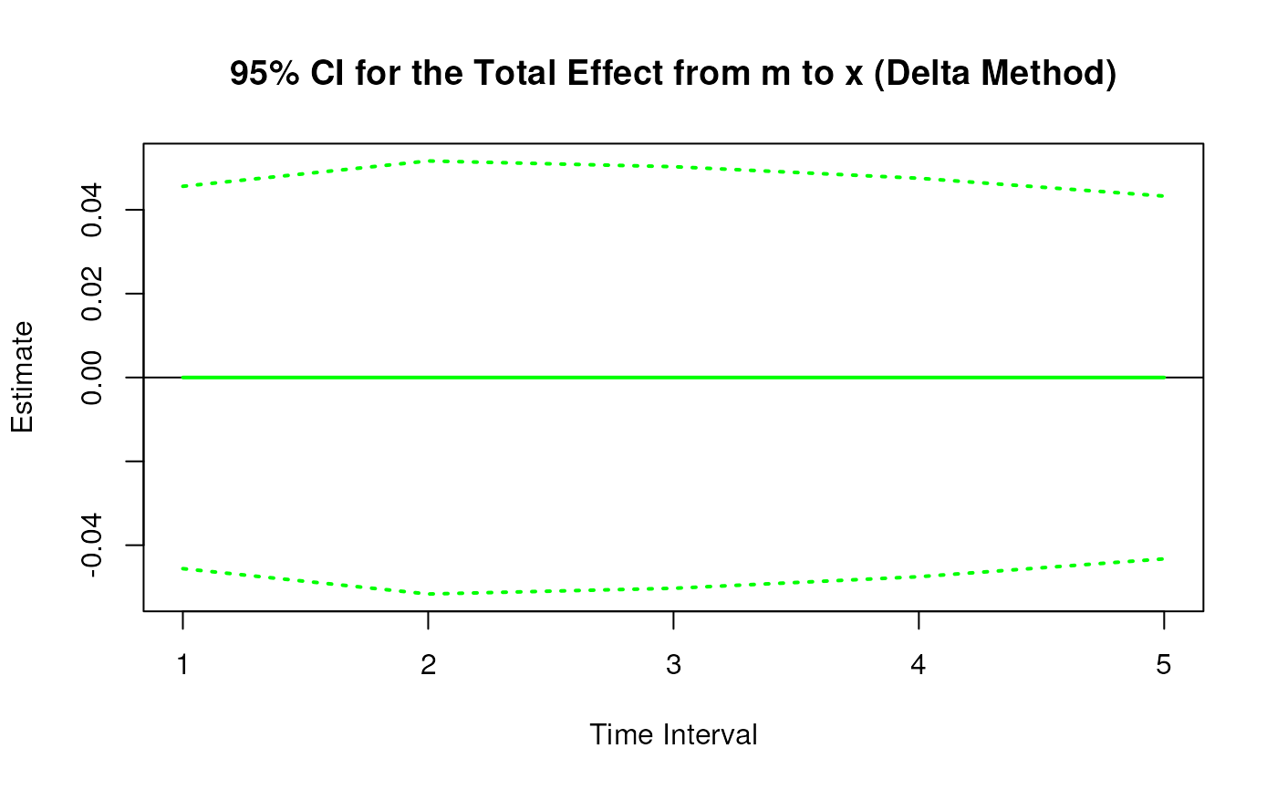
#> 4 from m to x 1 0.0000 0.0435 0.0000 1.0000 -0.0852 0.0852
#> 5 from m to m 1 0.5999 0.0326 18.3826 0.0000 0.5359 0.6639
#> 6 from m to y 1 0.3998 0.0284 14.0593 0.0000 0.3441 0.4556
#> 7 from y to x 1 0.0000 0.0418 0.0000 1.0000 -0.0820 0.0820
#> 8 from y to m 1 0.0000 0.0311 0.0000 1.0000 -0.0609 0.0609
#> 9 from y to y 1 0.5001 0.0274 18.2776 0.0000 0.4464 0.5537
#> 10 from x to x 2 0.4897 0.0548 8.9377 0.0000 0.3823 0.5971
#> 11 from x to m 2 0.6499 0.0537 12.1023 0.0000 0.5446 0.7551
#> 12 from x to y 2 0.0799 0.0342 2.3337 0.0196 0.0128 0.1470
#> 13 from m to x 2 0.0000 0.0513 0.0000 1.0000 -0.1006 0.1006
#> 14 from m to m 2 0.3599 0.0504 7.1405 0.0000 0.2611 0.4587
#> 15 from m to y 2 0.4398 0.0324 13.5818 0.0000 0.3763 0.5033
#> 16 from y to x 2 0.0000 0.0502 0.0000 1.0000 -0.0983 0.0983
#> 17 from y to m 2 0.0000 0.0493 0.0000 1.0000 -0.0967 0.0967
#> 18 from y to y 2 0.2501 0.0318 7.8668 0.0000 0.1878 0.3124
#> 19 from x to x 3 0.3427 0.0546 6.2779 0.0000 0.2357 0.4496
#> 20 from x to m 3 0.6347 0.0653 9.7126 0.0000 0.5066 0.7628
#> 21 from x to y 3 0.2508 0.0353 7.1106 0.0000 0.1817 0.3199
#> 22 from m to x 3 0.0000 0.0498 0.0000 1.0000 -0.0976 0.0976
#> 23 from m to m 3 0.2159 0.0609 3.5452 0.0004 0.0965 0.3352
#> 24 from m to y 3 0.3638 0.0325 11.1960 0.0000 0.3001 0.4275
#> 25 from y to x 3 0.0000 0.0456 0.0000 1.0000 -0.0893 0.0893
#> 26 from y to m 3 0.0000 0.0587 0.0000 1.0000 -0.1151 0.1151
#> 27 from y to y 3 0.1251 0.0299 4.1799 0.0000 0.0664 0.1837
#> 28 from x to x 4 0.2398 0.0536 4.4747 0.0000 0.1348 0.3448
#> 29 from x to m 4 0.5521 0.0717 7.7014 0.0000 0.4116 0.6926
#> 30 from x to y 4 0.3449 0.0394 8.7512 0.0000 0.2677 0.4222
#> 31 from m to x 4 0.0000 0.0456 0.0000 1.0000 -0.0894 0.0894
#> 32 from m to m 4 0.1295 0.0650 1.9937 0.0462 0.0022 0.2568
#> 33 from m to y 4 0.2683 0.0350 7.6627 0.0000 0.1996 0.3369
#> 34 from y to x 4 0.0000 0.0371 0.0000 1.0000 -0.0727 0.0727
#> 35 from y to m 4 0.0000 0.0599 0.0000 1.0000 -0.1174 0.1174
#> 36 from y to y 4 0.0625 0.0310 2.0161 0.0438 0.0017 0.1233
#> 37 from x to x 5 0.1678 0.0527 3.1821 0.0015 0.0644 0.2712
#> 38 from x to m 5 0.4511 0.0749 6.0254 0.0000 0.3044 0.5978
#> 39 from x to y 5 0.3693 0.0441 8.3649 0.0000 0.2827 0.4558
#> 40 from m to x 5 0.0000 0.0401 0.0000 1.0000 -0.0786 0.0786
#> 41 from m to m 5 0.0777 0.0642 1.2092 0.2266 -0.0482 0.2036
#> 42 from m to y 5 0.1859 0.0381 4.8780 0.0000 0.1112 0.2606
#> 43 from y to x 5 0.0000 0.0286 0.0000 1.0000 -0.0560 0.0560
#> 44 from y to m 5 0.0000 0.0554 0.0000 1.0000 -0.1086 0.1086
#> 45 from y to y 5 0.0313 0.0341 0.9180 0.3586 -0.0355 0.0980
summary(delta)
#> Call:
#> DeltaBeta(phi = phi, vcov_phi_vec = vcov_phi_vec, delta_t = 1:5)
#>
#> Elements of the matrix of lagged coefficients
#>
#> effect interval est se z p 2.5% 97.5%
#> 1 from x to x 1 0.6998 0.0471 14.8688 0.0000 0.6075 0.7920
#> 2 from x to m 1 0.5000 0.0352 14.1965 0.0000 0.4310 0.5691
#> 3 from x to y 1 -0.1000 0.0306 -3.2703 0.0011 -0.1600 -0.0401
#> 4 from m to x 1 0.0000 0.0435 0.0000 1.0000 -0.0852 0.0852
#> 5 from m to m 1 0.5999 0.0326 18.3826 0.0000 0.5359 0.6639
#> 6 from m to y 1 0.3998 0.0284 14.0593 0.0000 0.3441 0.4556
#> 7 from y to x 1 0.0000 0.0418 0.0000 1.0000 -0.0820 0.0820
#> 8 from y to m 1 0.0000 0.0311 0.0000 1.0000 -0.0609 0.0609
#> 9 from y to y 1 0.5001 0.0274 18.2776 0.0000 0.4464 0.5537
#> 10 from x to x 2 0.4897 0.0548 8.9377 0.0000 0.3823 0.5971
#> 11 from x to m 2 0.6499 0.0537 12.1023 0.0000 0.5446 0.7551
#> 12 from x to y 2 0.0799 0.0342 2.3337 0.0196 0.0128 0.1470
#> 13 from m to x 2 0.0000 0.0513 0.0000 1.0000 -0.1006 0.1006
#> 14 from m to m 2 0.3599 0.0504 7.1405 0.0000 0.2611 0.4587
#> 15 from m to y 2 0.4398 0.0324 13.5818 0.0000 0.3763 0.5033
#> 16 from y to x 2 0.0000 0.0502 0.0000 1.0000 -0.0983 0.0983
#> 17 from y to m 2 0.0000 0.0493 0.0000 1.0000 -0.0967 0.0967
#> 18 from y to y 2 0.2501 0.0318 7.8668 0.0000 0.1878 0.3124
#> 19 from x to x 3 0.3427 0.0546 6.2779 0.0000 0.2357 0.4496
#> 20 from x to m 3 0.6347 0.0653 9.7126 0.0000 0.5066 0.7628
#> 21 from x to y 3 0.2508 0.0353 7.1106 0.0000 0.1817 0.3199
#> 22 from m to x 3 0.0000 0.0498 0.0000 1.0000 -0.0976 0.0976
#> 23 from m to m 3 0.2159 0.0609 3.5452 0.0004 0.0965 0.3352
#> 24 from m to y 3 0.3638 0.0325 11.1960 0.0000 0.3001 0.4275
#> 25 from y to x 3 0.0000 0.0456 0.0000 1.0000 -0.0893 0.0893
#> 26 from y to m 3 0.0000 0.0587 0.0000 1.0000 -0.1151 0.1151
#> 27 from y to y 3 0.1251 0.0299 4.1799 0.0000 0.0664 0.1837
#> 28 from x to x 4 0.2398 0.0536 4.4747 0.0000 0.1348 0.3448
#> 29 from x to m 4 0.5521 0.0717 7.7014 0.0000 0.4116 0.6926
#> 30 from x to y 4 0.3449 0.0394 8.7512 0.0000 0.2677 0.4222
#> 31 from m to x 4 0.0000 0.0456 0.0000 1.0000 -0.0894 0.0894
#> 32 from m to m 4 0.1295 0.0650 1.9937 0.0462 0.0022 0.2568
#> 33 from m to y 4 0.2683 0.0350 7.6627 0.0000 0.1996 0.3369
#> 34 from y to x 4 0.0000 0.0371 0.0000 1.0000 -0.0727 0.0727
#> 35 from y to m 4 0.0000 0.0599 0.0000 1.0000 -0.1174 0.1174
#> 36 from y to y 4 0.0625 0.0310 2.0161 0.0438 0.0017 0.1233
#> 37 from x to x 5 0.1678 0.0527 3.1821 0.0015 0.0644 0.2712
#> 38 from x to m 5 0.4511 0.0749 6.0254 0.0000 0.3044 0.5978
#> 39 from x to y 5 0.3693 0.0441 8.3649 0.0000 0.2827 0.4558
#> 40 from m to x 5 0.0000 0.0401 0.0000 1.0000 -0.0786 0.0786
#> 41 from m to m 5 0.0777 0.0642 1.2092 0.2266 -0.0482 0.2036
#> 42 from m to y 5 0.1859 0.0381 4.8780 0.0000 0.1112 0.2606
#> 43 from y to x 5 0.0000 0.0286 0.0000 1.0000 -0.0560 0.0560
#> 44 from y to m 5 0.0000 0.0554 0.0000 1.0000 -0.1086 0.1086
#> 45 from y to y 5 0.0313 0.0341 0.9180 0.3586 -0.0355 0.0980
confint(delta, level = 0.95)
#> effect interval 2.5 % 97.5 %
#> 1 from x to x 1 0.607530630 0.79201437
#> 2 from x to m 1 0.430999370 0.56906888
#> 3 from x to y 1 -0.159994521 -0.04008223
#> 4 from m to x 1 -0.085180722 0.08518072
#> 5 from m to m 1 0.535934031 0.66385674
#> 6 from m to y 1 0.344095782 0.45557546
#> 7 from y to x 1 -0.081957196 0.08195720
#> 8 from y to m 1 -0.060893928 0.06089393
#> 9 from y to y 1 0.446449155 0.55369804
#> 10 from x to x 2 0.382298845 0.59706425
#> 11 from x to m 2 0.544630905 0.75512568
#> 12 from x to y 2 0.012796105 0.14700550
#> 13 from m to x 2 -0.100621301 0.10062130
#> 14 from m to m 2 0.261093683 0.45865526
#> 15 from m to y 2 0.376339257 0.50327430
#> 16 from y to x 2 -0.098336021 0.09833602
#> 17 from y to m 2 -0.096703960 0.09670396
#> 18 from y to y 2 0.187769671 0.31237753
#> 19 from x to x 3 0.235686018 0.44964534
#> 20 from x to m 3 0.506633055 0.76279989
#> 21 from x to y 3 0.181679901 0.31994775
#> 22 from m to x 3 -0.097647963 0.09764796
#> 23 from m to m 3 0.096535451 0.33523862
#> 24 from m to y 3 0.300134940 0.42751784
#> 25 from y to x 3 -0.089308174 0.08930817
#> 26 from y to m 3 -0.115121991 0.11512199
#> 27 from y to y 3 0.066417023 0.18369339
#> 28 from x to x 4 0.134758701 0.34481734
#> 29 from x to m 4 0.411600436 0.69261559
#> 30 from x to y 4 0.267675671 0.42218015
#> 31 from m to x 4 -0.089399053 0.08939905
#> 32 from m to m 4 0.002192406 0.25682686
#> 33 from m to y 4 0.199644090 0.33687451
#> 34 from y to x 4 -0.072744578 0.07274458
#> 35 from y to m 4 -0.117422876 0.11742288
#> 36 from y to y 4 0.001740919 0.12333269
#> 37 from x to x 5 0.064444048 0.27115007
#> 38 from x to m 5 0.304371874 0.59784661
#> 39 from x to y 5 0.282734719 0.45577286
#> 40 from m to x 5 -0.078617114 0.07861711
#> 41 from m to m 5 -0.048232879 0.20361734
#> 42 from m to y 5 0.111225188 0.26063873
#> 43 from y to x 5 -0.056029996 0.05603000
#> 44 from y to m 5 -0.108615295 0.10861530
#> 45 from y to y 5 -0.035495583 0.09804159
plot(delta)
# Methods -------------------------------------------------------------------
# DeltaBeta has a number of methods including
# print, summary, confint, and plot
print(delta)
#> Call:
#> DeltaBeta(phi = phi, vcov_phi_vec = vcov_phi_vec, delta_t = 1:5)
#>
#> Elements of the matrix of lagged coefficients
#>
#> effect interval est se z p 2.5% 97.5%
#> 1 from x to x 1 0.6998 0.0471 14.8688 0.0000 0.6075 0.7920
#> 2 from x to m 1 0.5000 0.0352 14.1965 0.0000 0.4310 0.5691
#> 3 from x to y 1 -0.1000 0.0306 -3.2703 0.0011 -0.1600 -0.0401
#> 4 from m to x 1 0.0000 0.0435 0.0000 1.0000 -0.0852 0.0852
#> 5 from m to m 1 0.5999 0.0326 18.3826 0.0000 0.5359 0.6639
#> 6 from m to y 1 0.3998 0.0284 14.0593 0.0000 0.3441 0.4556
#> 7 from y to x 1 0.0000 0.0418 0.0000 1.0000 -0.0820 0.0820
#> 8 from y to m 1 0.0000 0.0311 0.0000 1.0000 -0.0609 0.0609
#> 9 from y to y 1 0.5001 0.0274 18.2776 0.0000 0.4464 0.5537
#> 10 from x to x 2 0.4897 0.0548 8.9377 0.0000 0.3823 0.5971
#> 11 from x to m 2 0.6499 0.0537 12.1023 0.0000 0.5446 0.7551
#> 12 from x to y 2 0.0799 0.0342 2.3337 0.0196 0.0128 0.1470
#> 13 from m to x 2 0.0000 0.0513 0.0000 1.0000 -0.1006 0.1006
#> 14 from m to m 2 0.3599 0.0504 7.1405 0.0000 0.2611 0.4587
#> 15 from m to y 2 0.4398 0.0324 13.5818 0.0000 0.3763 0.5033
#> 16 from y to x 2 0.0000 0.0502 0.0000 1.0000 -0.0983 0.0983
#> 17 from y to m 2 0.0000 0.0493 0.0000 1.0000 -0.0967 0.0967
#> 18 from y to y 2 0.2501 0.0318 7.8668 0.0000 0.1878 0.3124
#> 19 from x to x 3 0.3427 0.0546 6.2779 0.0000 0.2357 0.4496
#> 20 from x to m 3 0.6347 0.0653 9.7126 0.0000 0.5066 0.7628
#> 21 from x to y 3 0.2508 0.0353 7.1106 0.0000 0.1817 0.3199
#> 22 from m to x 3 0.0000 0.0498 0.0000 1.0000 -0.0976 0.0976
#> 23 from m to m 3 0.2159 0.0609 3.5452 0.0004 0.0965 0.3352
#> 24 from m to y 3 0.3638 0.0325 11.1960 0.0000 0.3001 0.4275
#> 25 from y to x 3 0.0000 0.0456 0.0000 1.0000 -0.0893 0.0893
#> 26 from y to m 3 0.0000 0.0587 0.0000 1.0000 -0.1151 0.1151
#> 27 from y to y 3 0.1251 0.0299 4.1799 0.0000 0.0664 0.1837
#> 28 from x to x 4 0.2398 0.0536 4.4747 0.0000 0.1348 0.3448
#> 29 from x to m 4 0.5521 0.0717 7.7014 0.0000 0.4116 0.6926
#> 30 from x to y 4 0.3449 0.0394 8.7512 0.0000 0.2677 0.4222
#> 31 from m to x 4 0.0000 0.0456 0.0000 1.0000 -0.0894 0.0894
#> 32 from m to m 4 0.1295 0.0650 1.9937 0.0462 0.0022 0.2568
#> 33 from m to y 4 0.2683 0.0350 7.6627 0.0000 0.1996 0.3369
#> 34 from y to x 4 0.0000 0.0371 0.0000 1.0000 -0.0727 0.0727
#> 35 from y to m 4 0.0000 0.0599 0.0000 1.0000 -0.1174 0.1174
#> 36 from y to y 4 0.0625 0.0310 2.0161 0.0438 0.0017 0.1233
#> 37 from x to x 5 0.1678 0.0527 3.1821 0.0015 0.0644 0.2712
#> 38 from x to m 5 0.4511 0.0749 6.0254 0.0000 0.3044 0.5978
#> 39 from x to y 5 0.3693 0.0441 8.3649 0.0000 0.2827 0.4558
#> 40 from m to x 5 0.0000 0.0401 0.0000 1.0000 -0.0786 0.0786
#> 41 from m to m 5 0.0777 0.0642 1.2092 0.2266 -0.0482 0.2036
#> 42 from m to y 5 0.1859 0.0381 4.8780 0.0000 0.1112 0.2606
#> 43 from y to x 5 0.0000 0.0286 0.0000 1.0000 -0.0560 0.0560
#> 44 from y to m 5 0.0000 0.0554 0.0000 1.0000 -0.1086 0.1086
#> 45 from y to y 5 0.0313 0.0341 0.9180 0.3586 -0.0355 0.0980
summary(delta)
#> Call:
#> DeltaBeta(phi = phi, vcov_phi_vec = vcov_phi_vec, delta_t = 1:5)
#>
#> Elements of the matrix of lagged coefficients
#>
#> effect interval est se z p 2.5% 97.5%
#> 1 from x to x 1 0.6998 0.0471 14.8688 0.0000 0.6075 0.7920
#> 2 from x to m 1 0.5000 0.0352 14.1965 0.0000 0.4310 0.5691
#> 3 from x to y 1 -0.1000 0.0306 -3.2703 0.0011 -0.1600 -0.0401
#> 4 from m to x 1 0.0000 0.0435 0.0000 1.0000 -0.0852 0.0852
#> 5 from m to m 1 0.5999 0.0326 18.3826 0.0000 0.5359 0.6639
#> 6 from m to y 1 0.3998 0.0284 14.0593 0.0000 0.3441 0.4556
#> 7 from y to x 1 0.0000 0.0418 0.0000 1.0000 -0.0820 0.0820
#> 8 from y to m 1 0.0000 0.0311 0.0000 1.0000 -0.0609 0.0609
#> 9 from y to y 1 0.5001 0.0274 18.2776 0.0000 0.4464 0.5537
#> 10 from x to x 2 0.4897 0.0548 8.9377 0.0000 0.3823 0.5971
#> 11 from x to m 2 0.6499 0.0537 12.1023 0.0000 0.5446 0.7551
#> 12 from x to y 2 0.0799 0.0342 2.3337 0.0196 0.0128 0.1470
#> 13 from m to x 2 0.0000 0.0513 0.0000 1.0000 -0.1006 0.1006
#> 14 from m to m 2 0.3599 0.0504 7.1405 0.0000 0.2611 0.4587
#> 15 from m to y 2 0.4398 0.0324 13.5818 0.0000 0.3763 0.5033
#> 16 from y to x 2 0.0000 0.0502 0.0000 1.0000 -0.0983 0.0983
#> 17 from y to m 2 0.0000 0.0493 0.0000 1.0000 -0.0967 0.0967
#> 18 from y to y 2 0.2501 0.0318 7.8668 0.0000 0.1878 0.3124
#> 19 from x to x 3 0.3427 0.0546 6.2779 0.0000 0.2357 0.4496
#> 20 from x to m 3 0.6347 0.0653 9.7126 0.0000 0.5066 0.7628
#> 21 from x to y 3 0.2508 0.0353 7.1106 0.0000 0.1817 0.3199
#> 22 from m to x 3 0.0000 0.0498 0.0000 1.0000 -0.0976 0.0976
#> 23 from m to m 3 0.2159 0.0609 3.5452 0.0004 0.0965 0.3352
#> 24 from m to y 3 0.3638 0.0325 11.1960 0.0000 0.3001 0.4275
#> 25 from y to x 3 0.0000 0.0456 0.0000 1.0000 -0.0893 0.0893
#> 26 from y to m 3 0.0000 0.0587 0.0000 1.0000 -0.1151 0.1151
#> 27 from y to y 3 0.1251 0.0299 4.1799 0.0000 0.0664 0.1837
#> 28 from x to x 4 0.2398 0.0536 4.4747 0.0000 0.1348 0.3448
#> 29 from x to m 4 0.5521 0.0717 7.7014 0.0000 0.4116 0.6926
#> 30 from x to y 4 0.3449 0.0394 8.7512 0.0000 0.2677 0.4222
#> 31 from m to x 4 0.0000 0.0456 0.0000 1.0000 -0.0894 0.0894
#> 32 from m to m 4 0.1295 0.0650 1.9937 0.0462 0.0022 0.2568
#> 33 from m to y 4 0.2683 0.0350 7.6627 0.0000 0.1996 0.3369
#> 34 from y to x 4 0.0000 0.0371 0.0000 1.0000 -0.0727 0.0727
#> 35 from y to m 4 0.0000 0.0599 0.0000 1.0000 -0.1174 0.1174
#> 36 from y to y 4 0.0625 0.0310 2.0161 0.0438 0.0017 0.1233
#> 37 from x to x 5 0.1678 0.0527 3.1821 0.0015 0.0644 0.2712
#> 38 from x to m 5 0.4511 0.0749 6.0254 0.0000 0.3044 0.5978
#> 39 from x to y 5 0.3693 0.0441 8.3649 0.0000 0.2827 0.4558
#> 40 from m to x 5 0.0000 0.0401 0.0000 1.0000 -0.0786 0.0786
#> 41 from m to m 5 0.0777 0.0642 1.2092 0.2266 -0.0482 0.2036
#> 42 from m to y 5 0.1859 0.0381 4.8780 0.0000 0.1112 0.2606
#> 43 from y to x 5 0.0000 0.0286 0.0000 1.0000 -0.0560 0.0560
#> 44 from y to m 5 0.0000 0.0554 0.0000 1.0000 -0.1086 0.1086
#> 45 from y to y 5 0.0313 0.0341 0.9180 0.3586 -0.0355 0.0980
confint(delta, level = 0.95)
#> effect interval 2.5 % 97.5 %
#> 1 from x to x 1 0.607530630 0.79201437
#> 2 from x to m 1 0.430999370 0.56906888
#> 3 from x to y 1 -0.159994521 -0.04008223
#> 4 from m to x 1 -0.085180722 0.08518072
#> 5 from m to m 1 0.535934031 0.66385674
#> 6 from m to y 1 0.344095782 0.45557546
#> 7 from y to x 1 -0.081957196 0.08195720
#> 8 from y to m 1 -0.060893928 0.06089393
#> 9 from y to y 1 0.446449155 0.55369804
#> 10 from x to x 2 0.382298845 0.59706425
#> 11 from x to m 2 0.544630905 0.75512568
#> 12 from x to y 2 0.012796105 0.14700550
#> 13 from m to x 2 -0.100621301 0.10062130
#> 14 from m to m 2 0.261093683 0.45865526
#> 15 from m to y 2 0.376339257 0.50327430
#> 16 from y to x 2 -0.098336021 0.09833602
#> 17 from y to m 2 -0.096703960 0.09670396
#> 18 from y to y 2 0.187769671 0.31237753
#> 19 from x to x 3 0.235686018 0.44964534
#> 20 from x to m 3 0.506633055 0.76279989
#> 21 from x to y 3 0.181679901 0.31994775
#> 22 from m to x 3 -0.097647963 0.09764796
#> 23 from m to m 3 0.096535451 0.33523862
#> 24 from m to y 3 0.300134940 0.42751784
#> 25 from y to x 3 -0.089308174 0.08930817
#> 26 from y to m 3 -0.115121991 0.11512199
#> 27 from y to y 3 0.066417023 0.18369339
#> 28 from x to x 4 0.134758701 0.34481734
#> 29 from x to m 4 0.411600436 0.69261559
#> 30 from x to y 4 0.267675671 0.42218015
#> 31 from m to x 4 -0.089399053 0.08939905
#> 32 from m to m 4 0.002192406 0.25682686
#> 33 from m to y 4 0.199644090 0.33687451
#> 34 from y to x 4 -0.072744578 0.07274458
#> 35 from y to m 4 -0.117422876 0.11742288
#> 36 from y to y 4 0.001740919 0.12333269
#> 37 from x to x 5 0.064444048 0.27115007
#> 38 from x to m 5 0.304371874 0.59784661
#> 39 from x to y 5 0.282734719 0.45577286
#> 40 from m to x 5 -0.078617114 0.07861711
#> 41 from m to m 5 -0.048232879 0.20361734
#> 42 from m to y 5 0.111225188 0.26063873
#> 43 from y to x 5 -0.056029996 0.05603000
#> 44 from y to m 5 -0.108615295 0.10861530
#> 45 from y to y 5 -0.035495583 0.09804159
plot(delta)