Posterior Sampling Distribution for the Elements of the Matrix of Lagged Coefficients Over a Specific Time Interval or a Range of Time Intervals
Source:R/cTMed-posterior-beta.R
PosteriorBeta.RdThis function generates a posterior sampling distribution for the elements of the matrix of lagged coefficients \(\boldsymbol{\beta}\) over a specific time interval \(\Delta t\) or a range of time intervals using the first-order stochastic differential equation model drift matrix \(\boldsymbol{\Phi}\).
Arguments
- phi
List of numeric matrices. Each element of the list is a sample from the posterior distribution of the drift matrix (\(\boldsymbol{\Phi}\)). Each matrix should have row and column names pertaining to the variables in the system.
- delta_t
Numeric. Time interval (\(\Delta t\)).
- ncores
Positive integer. Number of cores to use. If
ncores = NULL, use a single core. Consider using multiple cores when number of replicationsRis a large value.- tol
Numeric. Smallest possible time interval to allow.
Value
Returns an object
of class ctmedmc which is a list with the following elements:
- call
Function call.
- args
Function arguments.
- fun
Function used ("PosteriorBeta").
- output
A list of length
length(delta_t).
Each element in the output list has the following elements:
- est
A vector of total, direct, and indirect effects.
- thetahatstar
A matrix of Monte Carlo total, direct, and indirect effects.
Details
See Total().
References
Bollen, K. A. (1987). Total, direct, and indirect effects in structural equation models. Sociological Methodology, 17, 37. doi:10.2307/271028
Deboeck, P. R., & Preacher, K. J. (2015). No need to be discrete: A method for continuous time mediation analysis. Structural Equation Modeling: A Multidisciplinary Journal, 23 (1), 61-75. doi:10.1080/10705511.2014.973960
Pesigan, I. J. A., Russell, M. A., & Chow, S.-M. (2025). Inferences and effect sizes for direct, indirect, and total effects in continuous-time mediation models. Psychological Methods. doi:10.1037/met0000779
Ryan, O., & Hamaker, E. L. (2021). Time to intervene: A continuous-time approach to network analysis and centrality. Psychometrika, 87 (1), 214-252. doi:10.1007/s11336-021-09767-0
See also
Other Continuous-Time Mediation Functions:
BootBeta(),
BootBetaStd(),
BootDirectCentral(),
BootDirectCentralStd(),
BootIndirectCentral(),
BootIndirectCentralStd(),
BootMed(),
BootMedStd(),
BootTotalCentral(),
BootTotalCentralStd(),
DeltaBeta(),
DeltaBetaStd(),
DeltaDirectCentral(),
DeltaDirectCentralStd(),
DeltaIndirectCentral(),
DeltaMed(),
DeltaMedStd(),
DeltaTotalCentral(),
DeltaTotalCentralStd(),
Direct(),
DirectCentral(),
DirectCentralStd(),
DirectStd(),
Indirect(),
IndirectCentral(),
IndirectCentralStd(),
IndirectStd(),
MCBeta(),
MCBetaStd(),
MCDirectCentral(),
MCDirectCentralStd(),
MCIndirectCentral(),
MCIndirectCentralStd(),
MCMed(),
MCMedStd(),
MCPhi(),
MCPhiSigma(),
MCTotalCentral(),
MCTotalCentralStd(),
Med(),
MedStd(),
PosteriorBetaStd(),
PosteriorDirectCentral(),
PosteriorDirectCentralStd(),
PosteriorIndirectCentral(),
PosteriorIndirectCentralStd(),
PosteriorMed(),
PosteriorMedStd(),
PosteriorTotalCentral(),
PosteriorTotalCentralStd(),
Total(),
TotalCentral(),
TotalCentralStd(),
TotalStd(),
Trajectory()
Examples
phi <- matrix(
data = c(
-0.357, 0.771, -0.450,
0.0, -0.511, 0.729,
0, 0, -0.693
),
nrow = 3
)
colnames(phi) <- rownames(phi) <- c("x", "m", "y")
vcov_phi_vec <- matrix(
data = c(
0.00843, 0.00040, -0.00151,
-0.00600, -0.00033, 0.00110,
0.00324, 0.00020, -0.00061,
0.00040, 0.00374, 0.00016,
-0.00022, -0.00273, -0.00016,
0.00009, 0.00150, 0.00012,
-0.00151, 0.00016, 0.00389,
0.00103, -0.00007, -0.00283,
-0.00050, 0.00000, 0.00156,
-0.00600, -0.00022, 0.00103,
0.00644, 0.00031, -0.00119,
-0.00374, -0.00021, 0.00070,
-0.00033, -0.00273, -0.00007,
0.00031, 0.00287, 0.00013,
-0.00014, -0.00170, -0.00012,
0.00110, -0.00016, -0.00283,
-0.00119, 0.00013, 0.00297,
0.00063, -0.00004, -0.00177,
0.00324, 0.00009, -0.00050,
-0.00374, -0.00014, 0.00063,
0.00495, 0.00024, -0.00093,
0.00020, 0.00150, 0.00000,
-0.00021, -0.00170, -0.00004,
0.00024, 0.00214, 0.00012,
-0.00061, 0.00012, 0.00156,
0.00070, -0.00012, -0.00177,
-0.00093, 0.00012, 0.00223
),
nrow = 9
)
phi <- MCPhi(
phi = phi,
vcov_phi_vec = vcov_phi_vec,
R = 1000L
)$output
# Specific time interval ----------------------------------------------------
PosteriorBeta(
phi = phi,
delta_t = 1
)
#> Call:
#> PosteriorBeta(phi = phi, delta_t = 1)
#>
#> Total, Direct, and Indirect Effects
#>
#> effect interval est se R 2.5% 97.5%
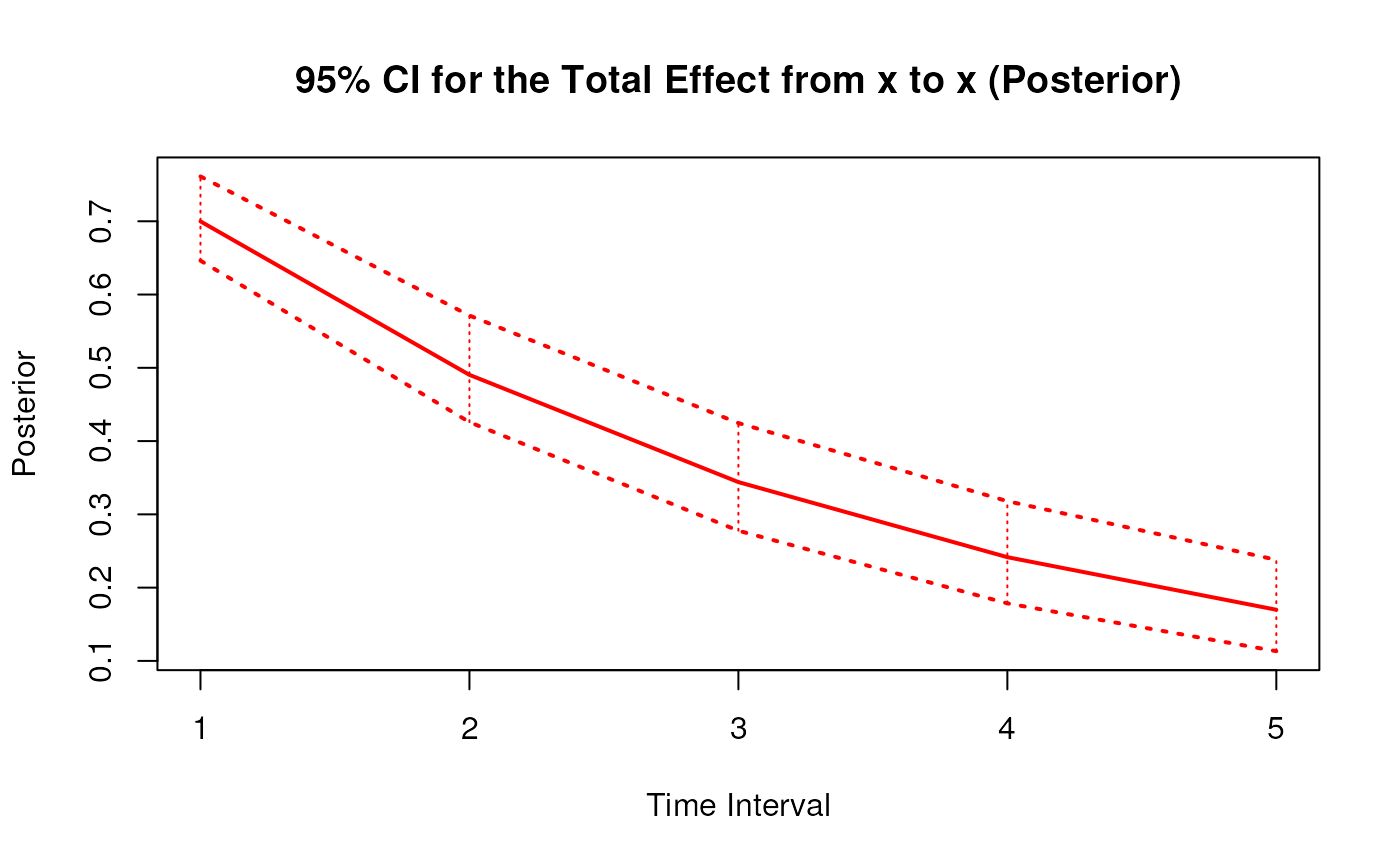
#> 1 from x to x 1 0.7005 0.0459 1000 0.6167 0.7991
#> 2 from x to m 1 0.4980 0.0350 1000 0.4344 0.5670
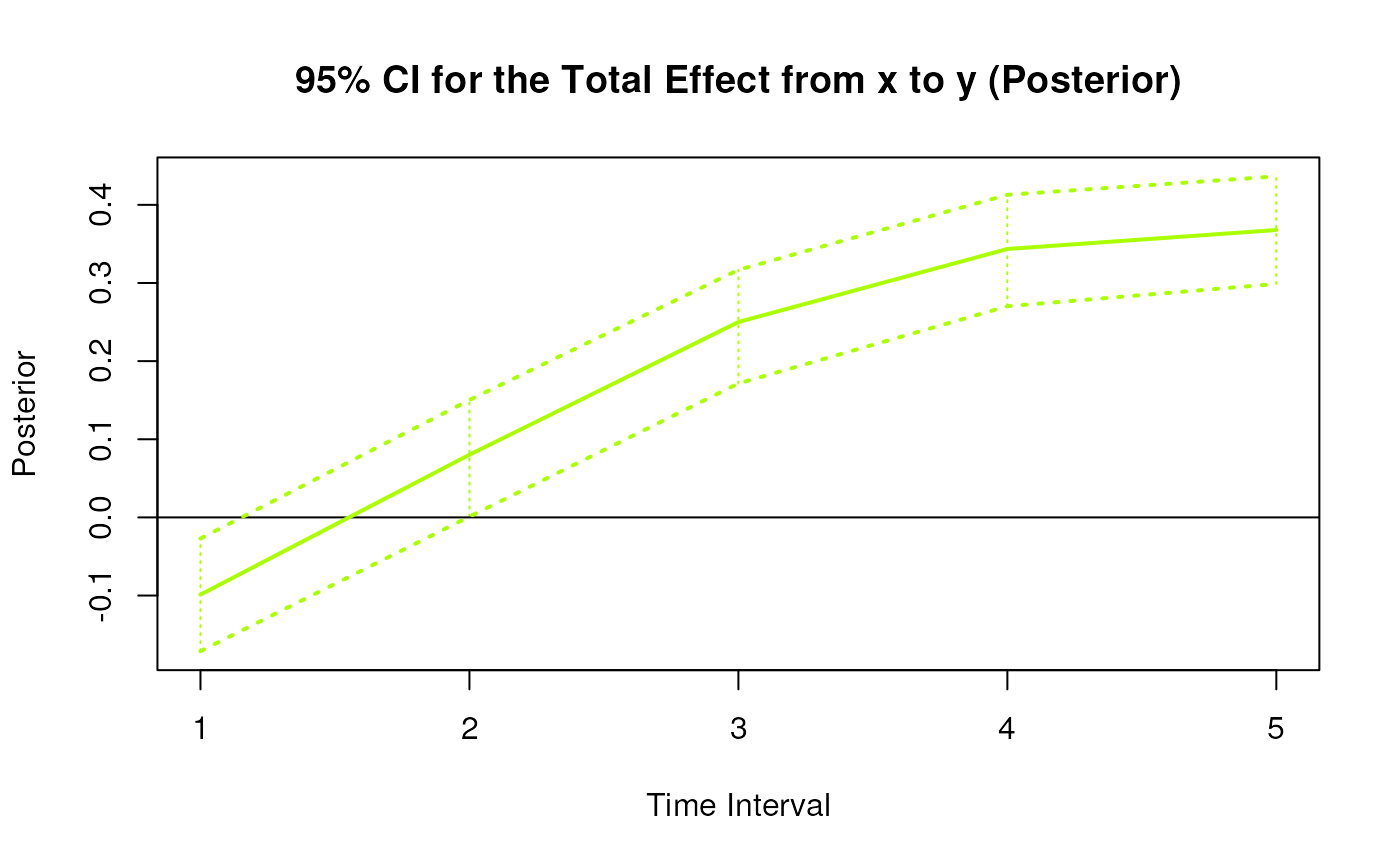
#> 3 from x to y 1 -0.1005 0.0305 1000 -0.1605 -0.0410
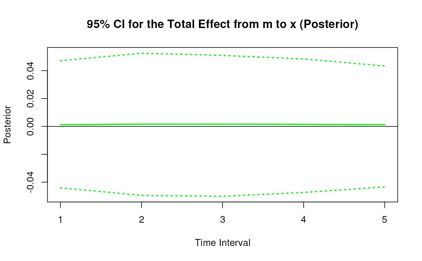
#> 4 from m to x 1 0.0016 0.0434 1000 -0.0825 0.0878
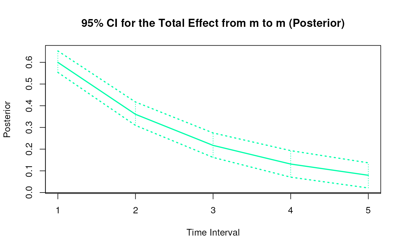
#> 5 from m to m 1 0.6016 0.0328 1000 0.5384 0.6645
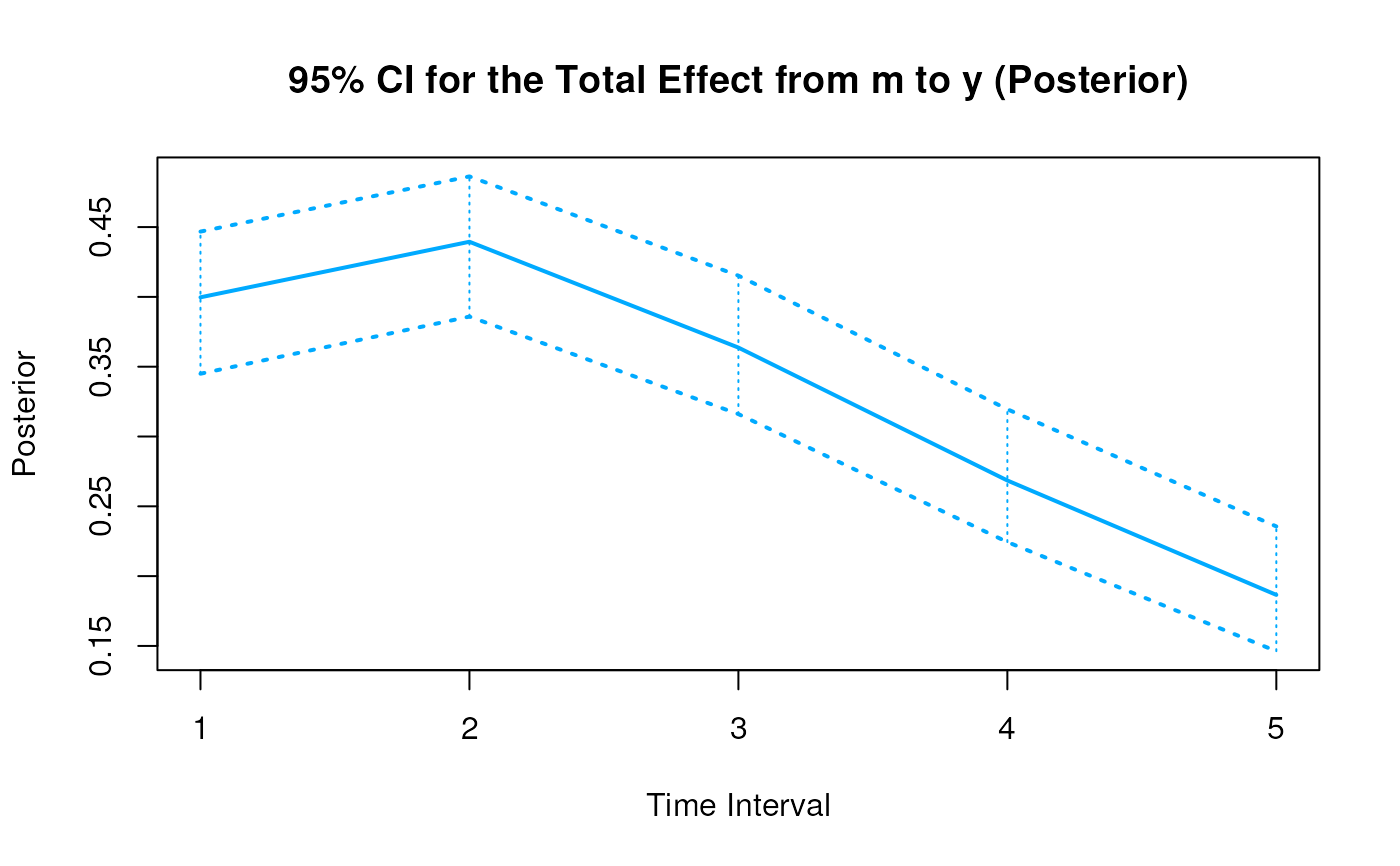
#> 6 from m to y 1 0.3994 0.0279 1000 0.3443 0.4513
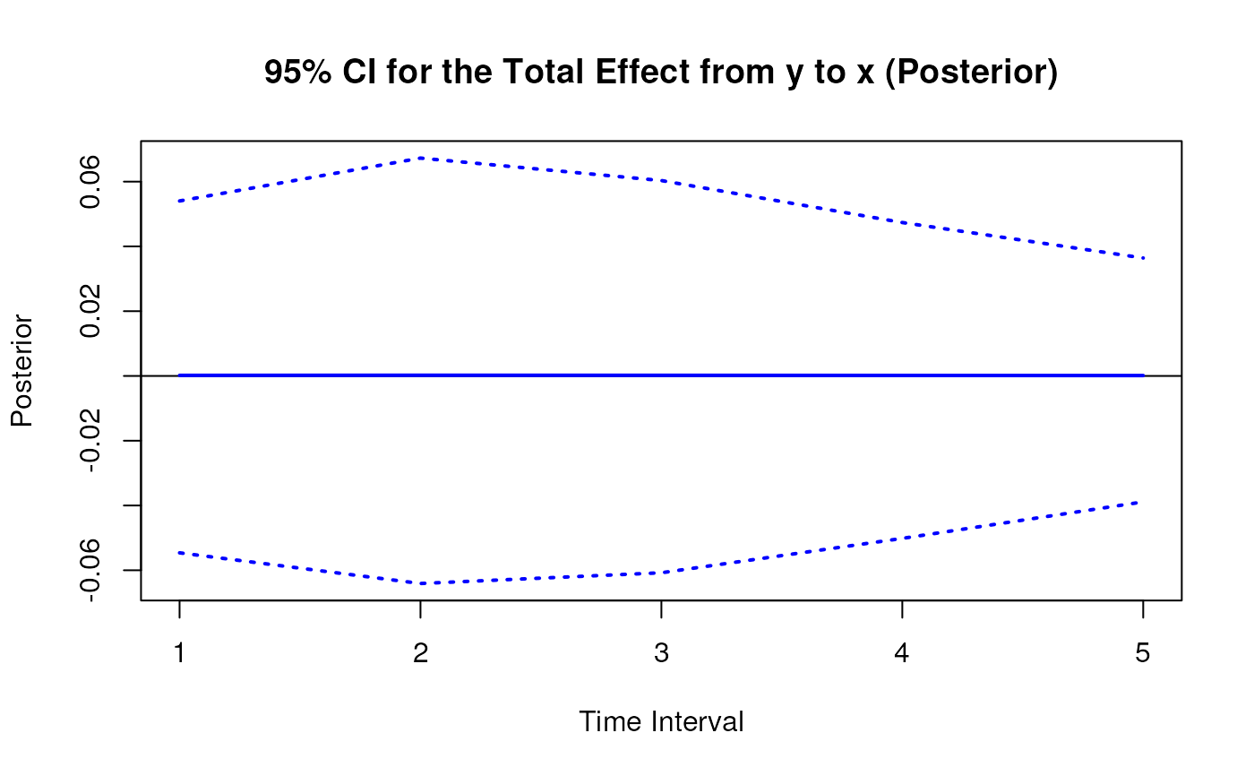
#> 7 from y to x 1 -0.0001 0.0419 1000 -0.0815 0.0808
#> 8 from y to m 1 -0.0008 0.0306 1000 -0.0579 0.0628
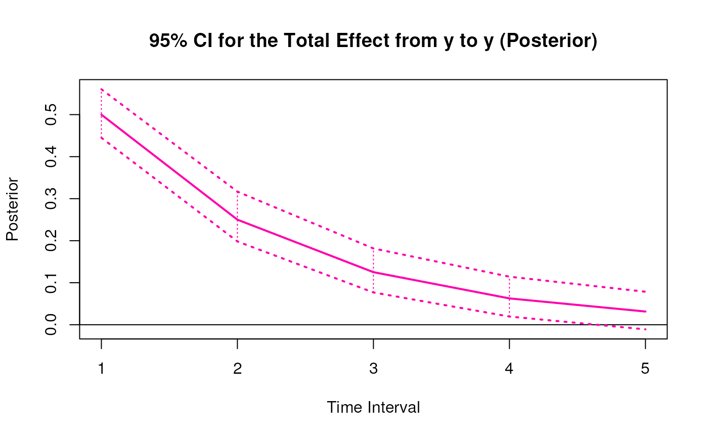
#> 9 from y to y 1 0.5001 0.0263 1000 0.4528 0.5541
# Range of time intervals ---------------------------------------------------
posterior <- PosteriorBeta(
phi = phi,
delta_t = 1:5
)
plot(posterior)


 # Methods -------------------------------------------------------------------
# PosteriorBeta has a number of methods including
# print, summary, confint, and plot
print(posterior)
#> Call:
#> PosteriorBeta(phi = phi, delta_t = 1:5)
#>
#> Total, Direct, and Indirect Effects
#>
#> effect interval est se R 2.5% 97.5%
#> 1 from x to x 1 0.7005 0.0459 1000 0.6167 0.7991
#> 2 from x to m 1 0.4980 0.0350 1000 0.4344 0.5670
#> 3 from x to y 1 -0.1005 0.0305 1000 -0.1605 -0.0410
#> 4 from m to x 1 0.0016 0.0434 1000 -0.0825 0.0878
#> 5 from m to m 1 0.6016 0.0328 1000 0.5384 0.6645
#> 6 from m to y 1 0.3994 0.0279 1000 0.3443 0.4513
#> 7 from y to x 1 -0.0001 0.0419 1000 -0.0815 0.0808
#> 8 from y to m 1 -0.0008 0.0306 1000 -0.0579 0.0628
#> 9 from y to y 1 0.5001 0.0263 1000 0.4528 0.5541
#> 10 from x to x 2 0.4915 0.0546 1000 0.3974 0.6171
#> 11 from x to m 2 0.6485 0.0528 1000 0.5512 0.7594
#> 12 from x to y 2 0.0783 0.0352 1000 0.0044 0.1435
#> 13 from m to x 2 0.0020 0.0520 1000 -0.1002 0.1037
#> 14 from m to m 2 0.3624 0.0504 1000 0.2620 0.4641
#> 15 from m to y 2 0.4399 0.0324 1000 0.3801 0.5049
#> 16 from y to x 2 -0.0001 0.0508 1000 -0.1006 0.0975
#> 17 from y to m 2 -0.0009 0.0493 1000 -0.0965 0.0971
#> 18 from y to y 2 0.2498 0.0305 1000 0.1939 0.3112
#> 19 from x to x 3 0.3453 0.0558 1000 0.2498 0.4727
#> 20 from x to m 3 0.6348 0.0651 1000 0.5213 0.7815
#> 21 from x to y 3 0.2488 0.0367 1000 0.1769 0.3219
#> 22 from m to x 3 0.0020 0.0514 1000 -0.1000 0.1005
#> 23 from m to m 3 0.2187 0.0610 1000 0.1009 0.3442
#> 24 from m to y 3 0.3645 0.0328 1000 0.3044 0.4282
#> 25 from y to x 3 -0.0001 0.0466 1000 -0.0937 0.0881
#> 26 from y to m 3 -0.0008 0.0593 1000 -0.1194 0.1145
#> 27 from y to y 3 0.1246 0.0288 1000 0.0714 0.1861
#> 28 from x to x 4 0.2429 0.0558 1000 0.1500 0.3691
#> 29 from x to m 4 0.5537 0.0728 1000 0.4286 0.7142
#> 30 from x to y 4 0.3433 0.0407 1000 0.2701 0.4262
#> 31 from m to x 4 0.0017 0.0479 1000 -0.0939 0.0980
#> 32 from m to m 4 0.1323 0.0658 1000 0.0055 0.2668
#> 33 from m to y 4 0.2695 0.0349 1000 0.2069 0.3396
#> 34 from y to x 4 -0.0001 0.0385 1000 -0.0768 0.0726
#> 35 from y to m 4 -0.0006 0.0611 1000 -0.1234 0.1144
#> 36 from y to y 4 0.0620 0.0305 1000 0.0051 0.1260
#> 37 from x to x 5 0.1710 0.0557 1000 0.0778 0.3024
#> 38 from x to m 5 0.4538 0.0773 1000 0.3228 0.6270
#> 39 from x to y 5 0.3684 0.0456 1000 0.2835 0.4685
#> 40 from m to x 5 0.0014 0.0428 1000 -0.0836 0.0903
#> 41 from m to m 5 0.0802 0.0660 1000 -0.0444 0.2158
#> 42 from m to y 5 0.1874 0.0376 1000 0.1157 0.2664
#> 43 from y to x 5 -0.0001 0.0303 1000 -0.0608 0.0586
#> 44 from y to m 5 -0.0005 0.0571 1000 -0.1163 0.1106
#> 45 from y to y 5 0.0308 0.0342 1000 -0.0339 0.1007
summary(posterior)
#> Call:
#> PosteriorBeta(phi = phi, delta_t = 1:5)
#>
#> Total, Direct, and Indirect Effects
#>
#> effect interval est se R 2.5% 97.5%
#> 1 from x to x 1 0.7005 0.0459 1000 0.6167 0.7991
#> 2 from x to m 1 0.4980 0.0350 1000 0.4344 0.5670
#> 3 from x to y 1 -0.1005 0.0305 1000 -0.1605 -0.0410
#> 4 from m to x 1 0.0016 0.0434 1000 -0.0825 0.0878
#> 5 from m to m 1 0.6016 0.0328 1000 0.5384 0.6645
#> 6 from m to y 1 0.3994 0.0279 1000 0.3443 0.4513
#> 7 from y to x 1 -0.0001 0.0419 1000 -0.0815 0.0808
#> 8 from y to m 1 -0.0008 0.0306 1000 -0.0579 0.0628
#> 9 from y to y 1 0.5001 0.0263 1000 0.4528 0.5541
#> 10 from x to x 2 0.4915 0.0546 1000 0.3974 0.6171
#> 11 from x to m 2 0.6485 0.0528 1000 0.5512 0.7594
#> 12 from x to y 2 0.0783 0.0352 1000 0.0044 0.1435
#> 13 from m to x 2 0.0020 0.0520 1000 -0.1002 0.1037
#> 14 from m to m 2 0.3624 0.0504 1000 0.2620 0.4641
#> 15 from m to y 2 0.4399 0.0324 1000 0.3801 0.5049
#> 16 from y to x 2 -0.0001 0.0508 1000 -0.1006 0.0975
#> 17 from y to m 2 -0.0009 0.0493 1000 -0.0965 0.0971
#> 18 from y to y 2 0.2498 0.0305 1000 0.1939 0.3112
#> 19 from x to x 3 0.3453 0.0558 1000 0.2498 0.4727
#> 20 from x to m 3 0.6348 0.0651 1000 0.5213 0.7815
#> 21 from x to y 3 0.2488 0.0367 1000 0.1769 0.3219
#> 22 from m to x 3 0.0020 0.0514 1000 -0.1000 0.1005
#> 23 from m to m 3 0.2187 0.0610 1000 0.1009 0.3442
#> 24 from m to y 3 0.3645 0.0328 1000 0.3044 0.4282
#> 25 from y to x 3 -0.0001 0.0466 1000 -0.0937 0.0881
#> 26 from y to m 3 -0.0008 0.0593 1000 -0.1194 0.1145
#> 27 from y to y 3 0.1246 0.0288 1000 0.0714 0.1861
#> 28 from x to x 4 0.2429 0.0558 1000 0.1500 0.3691
#> 29 from x to m 4 0.5537 0.0728 1000 0.4286 0.7142
#> 30 from x to y 4 0.3433 0.0407 1000 0.2701 0.4262
#> 31 from m to x 4 0.0017 0.0479 1000 -0.0939 0.0980
#> 32 from m to m 4 0.1323 0.0658 1000 0.0055 0.2668
#> 33 from m to y 4 0.2695 0.0349 1000 0.2069 0.3396
#> 34 from y to x 4 -0.0001 0.0385 1000 -0.0768 0.0726
#> 35 from y to m 4 -0.0006 0.0611 1000 -0.1234 0.1144
#> 36 from y to y 4 0.0620 0.0305 1000 0.0051 0.1260
#> 37 from x to x 5 0.1710 0.0557 1000 0.0778 0.3024
#> 38 from x to m 5 0.4538 0.0773 1000 0.3228 0.6270
#> 39 from x to y 5 0.3684 0.0456 1000 0.2835 0.4685
#> 40 from m to x 5 0.0014 0.0428 1000 -0.0836 0.0903
#> 41 from m to m 5 0.0802 0.0660 1000 -0.0444 0.2158
#> 42 from m to y 5 0.1874 0.0376 1000 0.1157 0.2664
#> 43 from y to x 5 -0.0001 0.0303 1000 -0.0608 0.0586
#> 44 from y to m 5 -0.0005 0.0571 1000 -0.1163 0.1106
#> 45 from y to y 5 0.0308 0.0342 1000 -0.0339 0.1007
confint(posterior, level = 0.95)
#> effect interval 2.5 % 97.5 %
#> 1 from x to x 1 0.616733974 0.79909822
#> 2 from x to m 1 0.434362221 0.56704068
#> 3 from x to y 1 -0.160466336 -0.04099099
#> 4 from m to x 1 -0.082547162 0.08781072
#> 5 from m to m 1 0.538436856 0.66453689
#> 6 from m to y 1 0.344285545 0.45127729
#> 7 from y to x 1 -0.081488237 0.08080213
#> 8 from y to m 1 -0.057914084 0.06275387
#> 9 from y to y 1 0.452763210 0.55412643
#> 10 from x to x 2 0.397363368 0.61706647
#> 11 from x to m 2 0.551242396 0.75943697
#> 12 from x to y 2 0.004384326 0.14349322
#> 13 from m to x 2 -0.100207649 0.10369542
#> 14 from m to m 2 0.262035619 0.46414611
#> 15 from m to y 2 0.380087785 0.50492632
#> 16 from y to x 2 -0.100560203 0.09751705
#> 17 from y to m 2 -0.096510078 0.09705996
#> 18 from y to y 2 0.193901260 0.31115718
#> 19 from x to x 3 0.249811049 0.47273056
#> 20 from x to m 3 0.521279120 0.78145826
#> 21 from x to y 3 0.176939533 0.32188069
#> 22 from m to x 3 -0.100046827 0.10049703
#> 23 from m to m 3 0.100861560 0.34415912
#> 24 from m to y 3 0.304375171 0.42818155
#> 25 from y to x 3 -0.093706942 0.08808043
#> 26 from y to m 3 -0.119394454 0.11448483
#> 27 from y to y 3 0.071403513 0.18605440
#> 28 from x to x 4 0.150024560 0.36907160
#> 29 from x to m 4 0.428596593 0.71424698
#> 30 from x to y 4 0.270116254 0.42616496
#> 31 from m to x 4 -0.093887342 0.09803768
#> 32 from m to m 4 0.005548960 0.26681974
#> 33 from m to y 4 0.206942676 0.33958857
#> 34 from y to x 4 -0.076811636 0.07264047
#> 35 from y to m 4 -0.123433377 0.11442935
#> 36 from y to y 4 0.005078871 0.12595826
#> 37 from x to x 5 0.077778773 0.30238314
#> 38 from x to m 5 0.322840631 0.62695796
#> 39 from x to y 5 0.283500487 0.46854501
#> 40 from m to x 5 -0.083578716 0.09033935
#> 41 from m to m 5 -0.044396900 0.21579508
#> 42 from m to y 5 0.115666004 0.26644885
#> 43 from y to x 5 -0.060790141 0.05857253
#> 44 from y to m 5 -0.116317805 0.11059869
#> 45 from y to y 5 -0.033923023 0.10067844
plot(posterior)
# Methods -------------------------------------------------------------------
# PosteriorBeta has a number of methods including
# print, summary, confint, and plot
print(posterior)
#> Call:
#> PosteriorBeta(phi = phi, delta_t = 1:5)
#>
#> Total, Direct, and Indirect Effects
#>
#> effect interval est se R 2.5% 97.5%
#> 1 from x to x 1 0.7005 0.0459 1000 0.6167 0.7991
#> 2 from x to m 1 0.4980 0.0350 1000 0.4344 0.5670
#> 3 from x to y 1 -0.1005 0.0305 1000 -0.1605 -0.0410
#> 4 from m to x 1 0.0016 0.0434 1000 -0.0825 0.0878
#> 5 from m to m 1 0.6016 0.0328 1000 0.5384 0.6645
#> 6 from m to y 1 0.3994 0.0279 1000 0.3443 0.4513
#> 7 from y to x 1 -0.0001 0.0419 1000 -0.0815 0.0808
#> 8 from y to m 1 -0.0008 0.0306 1000 -0.0579 0.0628
#> 9 from y to y 1 0.5001 0.0263 1000 0.4528 0.5541
#> 10 from x to x 2 0.4915 0.0546 1000 0.3974 0.6171
#> 11 from x to m 2 0.6485 0.0528 1000 0.5512 0.7594
#> 12 from x to y 2 0.0783 0.0352 1000 0.0044 0.1435
#> 13 from m to x 2 0.0020 0.0520 1000 -0.1002 0.1037
#> 14 from m to m 2 0.3624 0.0504 1000 0.2620 0.4641
#> 15 from m to y 2 0.4399 0.0324 1000 0.3801 0.5049
#> 16 from y to x 2 -0.0001 0.0508 1000 -0.1006 0.0975
#> 17 from y to m 2 -0.0009 0.0493 1000 -0.0965 0.0971
#> 18 from y to y 2 0.2498 0.0305 1000 0.1939 0.3112
#> 19 from x to x 3 0.3453 0.0558 1000 0.2498 0.4727
#> 20 from x to m 3 0.6348 0.0651 1000 0.5213 0.7815
#> 21 from x to y 3 0.2488 0.0367 1000 0.1769 0.3219
#> 22 from m to x 3 0.0020 0.0514 1000 -0.1000 0.1005
#> 23 from m to m 3 0.2187 0.0610 1000 0.1009 0.3442
#> 24 from m to y 3 0.3645 0.0328 1000 0.3044 0.4282
#> 25 from y to x 3 -0.0001 0.0466 1000 -0.0937 0.0881
#> 26 from y to m 3 -0.0008 0.0593 1000 -0.1194 0.1145
#> 27 from y to y 3 0.1246 0.0288 1000 0.0714 0.1861
#> 28 from x to x 4 0.2429 0.0558 1000 0.1500 0.3691
#> 29 from x to m 4 0.5537 0.0728 1000 0.4286 0.7142
#> 30 from x to y 4 0.3433 0.0407 1000 0.2701 0.4262
#> 31 from m to x 4 0.0017 0.0479 1000 -0.0939 0.0980
#> 32 from m to m 4 0.1323 0.0658 1000 0.0055 0.2668
#> 33 from m to y 4 0.2695 0.0349 1000 0.2069 0.3396
#> 34 from y to x 4 -0.0001 0.0385 1000 -0.0768 0.0726
#> 35 from y to m 4 -0.0006 0.0611 1000 -0.1234 0.1144
#> 36 from y to y 4 0.0620 0.0305 1000 0.0051 0.1260
#> 37 from x to x 5 0.1710 0.0557 1000 0.0778 0.3024
#> 38 from x to m 5 0.4538 0.0773 1000 0.3228 0.6270
#> 39 from x to y 5 0.3684 0.0456 1000 0.2835 0.4685
#> 40 from m to x 5 0.0014 0.0428 1000 -0.0836 0.0903
#> 41 from m to m 5 0.0802 0.0660 1000 -0.0444 0.2158
#> 42 from m to y 5 0.1874 0.0376 1000 0.1157 0.2664
#> 43 from y to x 5 -0.0001 0.0303 1000 -0.0608 0.0586
#> 44 from y to m 5 -0.0005 0.0571 1000 -0.1163 0.1106
#> 45 from y to y 5 0.0308 0.0342 1000 -0.0339 0.1007
summary(posterior)
#> Call:
#> PosteriorBeta(phi = phi, delta_t = 1:5)
#>
#> Total, Direct, and Indirect Effects
#>
#> effect interval est se R 2.5% 97.5%
#> 1 from x to x 1 0.7005 0.0459 1000 0.6167 0.7991
#> 2 from x to m 1 0.4980 0.0350 1000 0.4344 0.5670
#> 3 from x to y 1 -0.1005 0.0305 1000 -0.1605 -0.0410
#> 4 from m to x 1 0.0016 0.0434 1000 -0.0825 0.0878
#> 5 from m to m 1 0.6016 0.0328 1000 0.5384 0.6645
#> 6 from m to y 1 0.3994 0.0279 1000 0.3443 0.4513
#> 7 from y to x 1 -0.0001 0.0419 1000 -0.0815 0.0808
#> 8 from y to m 1 -0.0008 0.0306 1000 -0.0579 0.0628
#> 9 from y to y 1 0.5001 0.0263 1000 0.4528 0.5541
#> 10 from x to x 2 0.4915 0.0546 1000 0.3974 0.6171
#> 11 from x to m 2 0.6485 0.0528 1000 0.5512 0.7594
#> 12 from x to y 2 0.0783 0.0352 1000 0.0044 0.1435
#> 13 from m to x 2 0.0020 0.0520 1000 -0.1002 0.1037
#> 14 from m to m 2 0.3624 0.0504 1000 0.2620 0.4641
#> 15 from m to y 2 0.4399 0.0324 1000 0.3801 0.5049
#> 16 from y to x 2 -0.0001 0.0508 1000 -0.1006 0.0975
#> 17 from y to m 2 -0.0009 0.0493 1000 -0.0965 0.0971
#> 18 from y to y 2 0.2498 0.0305 1000 0.1939 0.3112
#> 19 from x to x 3 0.3453 0.0558 1000 0.2498 0.4727
#> 20 from x to m 3 0.6348 0.0651 1000 0.5213 0.7815
#> 21 from x to y 3 0.2488 0.0367 1000 0.1769 0.3219
#> 22 from m to x 3 0.0020 0.0514 1000 -0.1000 0.1005
#> 23 from m to m 3 0.2187 0.0610 1000 0.1009 0.3442
#> 24 from m to y 3 0.3645 0.0328 1000 0.3044 0.4282
#> 25 from y to x 3 -0.0001 0.0466 1000 -0.0937 0.0881
#> 26 from y to m 3 -0.0008 0.0593 1000 -0.1194 0.1145
#> 27 from y to y 3 0.1246 0.0288 1000 0.0714 0.1861
#> 28 from x to x 4 0.2429 0.0558 1000 0.1500 0.3691
#> 29 from x to m 4 0.5537 0.0728 1000 0.4286 0.7142
#> 30 from x to y 4 0.3433 0.0407 1000 0.2701 0.4262
#> 31 from m to x 4 0.0017 0.0479 1000 -0.0939 0.0980
#> 32 from m to m 4 0.1323 0.0658 1000 0.0055 0.2668
#> 33 from m to y 4 0.2695 0.0349 1000 0.2069 0.3396
#> 34 from y to x 4 -0.0001 0.0385 1000 -0.0768 0.0726
#> 35 from y to m 4 -0.0006 0.0611 1000 -0.1234 0.1144
#> 36 from y to y 4 0.0620 0.0305 1000 0.0051 0.1260
#> 37 from x to x 5 0.1710 0.0557 1000 0.0778 0.3024
#> 38 from x to m 5 0.4538 0.0773 1000 0.3228 0.6270
#> 39 from x to y 5 0.3684 0.0456 1000 0.2835 0.4685
#> 40 from m to x 5 0.0014 0.0428 1000 -0.0836 0.0903
#> 41 from m to m 5 0.0802 0.0660 1000 -0.0444 0.2158
#> 42 from m to y 5 0.1874 0.0376 1000 0.1157 0.2664
#> 43 from y to x 5 -0.0001 0.0303 1000 -0.0608 0.0586
#> 44 from y to m 5 -0.0005 0.0571 1000 -0.1163 0.1106
#> 45 from y to y 5 0.0308 0.0342 1000 -0.0339 0.1007
confint(posterior, level = 0.95)
#> effect interval 2.5 % 97.5 %
#> 1 from x to x 1 0.616733974 0.79909822
#> 2 from x to m 1 0.434362221 0.56704068
#> 3 from x to y 1 -0.160466336 -0.04099099
#> 4 from m to x 1 -0.082547162 0.08781072
#> 5 from m to m 1 0.538436856 0.66453689
#> 6 from m to y 1 0.344285545 0.45127729
#> 7 from y to x 1 -0.081488237 0.08080213
#> 8 from y to m 1 -0.057914084 0.06275387
#> 9 from y to y 1 0.452763210 0.55412643
#> 10 from x to x 2 0.397363368 0.61706647
#> 11 from x to m 2 0.551242396 0.75943697
#> 12 from x to y 2 0.004384326 0.14349322
#> 13 from m to x 2 -0.100207649 0.10369542
#> 14 from m to m 2 0.262035619 0.46414611
#> 15 from m to y 2 0.380087785 0.50492632
#> 16 from y to x 2 -0.100560203 0.09751705
#> 17 from y to m 2 -0.096510078 0.09705996
#> 18 from y to y 2 0.193901260 0.31115718
#> 19 from x to x 3 0.249811049 0.47273056
#> 20 from x to m 3 0.521279120 0.78145826
#> 21 from x to y 3 0.176939533 0.32188069
#> 22 from m to x 3 -0.100046827 0.10049703
#> 23 from m to m 3 0.100861560 0.34415912
#> 24 from m to y 3 0.304375171 0.42818155
#> 25 from y to x 3 -0.093706942 0.08808043
#> 26 from y to m 3 -0.119394454 0.11448483
#> 27 from y to y 3 0.071403513 0.18605440
#> 28 from x to x 4 0.150024560 0.36907160
#> 29 from x to m 4 0.428596593 0.71424698
#> 30 from x to y 4 0.270116254 0.42616496
#> 31 from m to x 4 -0.093887342 0.09803768
#> 32 from m to m 4 0.005548960 0.26681974
#> 33 from m to y 4 0.206942676 0.33958857
#> 34 from y to x 4 -0.076811636 0.07264047
#> 35 from y to m 4 -0.123433377 0.11442935
#> 36 from y to y 4 0.005078871 0.12595826
#> 37 from x to x 5 0.077778773 0.30238314
#> 38 from x to m 5 0.322840631 0.62695796
#> 39 from x to y 5 0.283500487 0.46854501
#> 40 from m to x 5 -0.083578716 0.09033935
#> 41 from m to m 5 -0.044396900 0.21579508
#> 42 from m to y 5 0.115666004 0.26644885
#> 43 from y to x 5 -0.060790141 0.05857253
#> 44 from y to m 5 -0.116317805 0.11059869
#> 45 from y to y 5 -0.033923023 0.10067844
plot(posterior)