Delta Method Sampling Variance-Covariance Matrix for the Total Effect Centrality Over a Specific Time Interval or a Range of Time Intervals
Source:R/cTMed-delta-total-central.R
DeltaTotalCentral.RdThis function computes the delta method sampling variance-covariance matrix for the total effect centrality over a specific time interval \(\Delta t\) or a range of time intervals using the first-order stochastic differential equation model's drift matrix \(\boldsymbol{\Phi}\).
Arguments
- phi
Numeric matrix. The drift matrix (\(\boldsymbol{\Phi}\)).
phishould have row and column names pertaining to the variables in the system.- vcov_phi_vec
Numeric matrix. The sampling variance-covariance matrix of \(\mathrm{vec} \left( \boldsymbol{\Phi} \right)\).
- delta_t
Vector of positive numbers. Time interval (\(\Delta t\)).
- ncores
Positive integer. Number of cores to use. If
ncores = NULL, use a single core. Consider using multiple cores when the length ofdelta_tis long.- tol
Numeric. Smallest possible time interval to allow.
Value
Returns an object
of class ctmeddelta which is a list with the following elements:
- call
Function call.
- args
Function arguments.
- fun
Function used ("DeltaTotalCentral").
- output
A list of length
length(delta_t).
Each element in the output list has the following elements:
- delta_t
Time interval.
- jacobian
Jacobian matrix.
- est
Estimated total effect centrality.
- vcov
Sampling variance-covariance matrix of estimated total effect centrality.
Details
See TotalCentral() for more details.
Delta Method
Let \(\boldsymbol{\theta}\) be \(\mathrm{vec} \left( \boldsymbol{\Phi} \right)\), that is, the elements of the \(\boldsymbol{\Phi}\) matrix in vector form sorted column-wise. Let \(\hat{\boldsymbol{\theta}}\) be \(\mathrm{vec} \left( \hat{\boldsymbol{\Phi}} \right)\). By the multivariate central limit theory, the function \(\mathbf{g}\) using \(\hat{\boldsymbol{\theta}}\) as input can be expressed as:
$$ \sqrt{n} \left( \mathbf{g} \left( \hat{\boldsymbol{\theta}} \right) - \mathbf{g} \left( \boldsymbol{\theta} \right) \right) \xrightarrow[]{ \mathrm{D} } \mathcal{N} \left( 0, \mathbf{J} \boldsymbol{\Gamma} \mathbf{J}^{\prime} \right) $$
where \(\mathbf{J}\) is the matrix of first-order derivatives of the function \(\mathbf{g}\) with respect to the elements of \(\boldsymbol{\theta}\) and \(\boldsymbol{\Gamma}\) is the asymptotic variance-covariance matrix of \(\hat{\boldsymbol{\theta}}\).
From the former, we can derive the distribution of \(\mathbf{g} \left( \hat{\boldsymbol{\theta}} \right)\) as follows:
$$ \mathbf{g} \left( \hat{\boldsymbol{\theta}} \right) \approx \mathcal{N} \left( \mathbf{g} \left( \boldsymbol{\theta} \right) , n^{-1} \mathbf{J} \boldsymbol{\Gamma} \mathbf{J}^{\prime} \right) $$
The uncertainty associated with the estimator \(\mathbf{g} \left( \hat{\boldsymbol{\theta}} \right)\) is, therefore, given by \(n^{-1} \mathbf{J} \boldsymbol{\Gamma} \mathbf{J}^{\prime}\) . When \(\boldsymbol{\Gamma}\) is unknown, by substitution, we can use the estimated sampling variance-covariance matrix of \(\hat{\boldsymbol{\theta}}\), that is, \(\hat{\mathbb{V}} \left( \hat{\boldsymbol{\theta}} \right)\) for \(n^{-1} \boldsymbol{\Gamma}\). Therefore, the sampling variance-covariance matrix of \(\mathbf{g} \left( \hat{\boldsymbol{\theta}} \right)\) is given by
$$ \mathbf{g} \left( \hat{\boldsymbol{\theta}} \right) \approx \mathcal{N} \left( \mathbf{g} \left( \boldsymbol{\theta} \right) , \mathbf{J} \hat{\mathbb{V}} \left( \hat{\boldsymbol{\theta}} \right) \mathbf{J}^{\prime} \right) . $$
References
Bollen, K. A. (1987). Total, direct, and indirect effects in structural equation models. Sociological Methodology, 17, 37. doi:10.2307/271028
Deboeck, P. R., & Preacher, K. J. (2015). No need to be discrete: A method for continuous time mediation analysis. Structural Equation Modeling: A Multidisciplinary Journal, 23 (1), 61-75. doi:10.1080/10705511.2014.973960
Pesigan, I. J. A., Russell, M. A., & Chow, S.-M. (2025). Inferences and effect sizes for direct, indirect, and total effects in continuous-time mediation models. Psychological Methods. doi:10.1037/met0000779
Ryan, O., & Hamaker, E. L. (2021). Time to intervene: A continuous-time approach to network analysis and centrality. Psychometrika, 87 (1), 214-252. doi:10.1007/s11336-021-09767-0
See also
Other Continuous-Time Mediation Functions:
BootBeta(),
BootBetaStd(),
BootDirectCentral(),
BootDirectCentralStd(),
BootIndirectCentral(),
BootIndirectCentralStd(),
BootMed(),
BootMedStd(),
BootTotalCentral(),
BootTotalCentralStd(),
DeltaBeta(),
DeltaBetaStd(),
DeltaDirectCentral(),
DeltaDirectCentralStd(),
DeltaIndirectCentral(),
DeltaMed(),
DeltaMedStd(),
DeltaTotalCentralStd(),
Direct(),
DirectCentral(),
DirectCentralStd(),
DirectStd(),
Indirect(),
IndirectCentral(),
IndirectCentralStd(),
IndirectStd(),
MCBeta(),
MCBetaStd(),
MCDirectCentral(),
MCDirectCentralStd(),
MCIndirectCentral(),
MCIndirectCentralStd(),
MCMed(),
MCMedStd(),
MCPhi(),
MCPhiSigma(),
MCTotalCentral(),
MCTotalCentralStd(),
Med(),
MedStd(),
PosteriorBeta(),
PosteriorBetaStd(),
PosteriorDirectCentral(),
PosteriorDirectCentralStd(),
PosteriorIndirectCentral(),
PosteriorIndirectCentralStd(),
PosteriorMed(),
PosteriorMedStd(),
PosteriorTotalCentral(),
PosteriorTotalCentralStd(),
Total(),
TotalCentral(),
TotalCentralStd(),
TotalStd(),
Trajectory()
Examples
phi <- matrix(
data = c(
-0.357, 0.771, -0.450,
0.0, -0.511, 0.729,
0, 0, -0.693
),
nrow = 3
)
colnames(phi) <- rownames(phi) <- c("x", "m", "y")
vcov_phi_vec <- matrix(
data = c(
0.00843, 0.00040, -0.00151,
-0.00600, -0.00033, 0.00110,
0.00324, 0.00020, -0.00061,
0.00040, 0.00374, 0.00016,
-0.00022, -0.00273, -0.00016,
0.00009, 0.00150, 0.00012,
-0.00151, 0.00016, 0.00389,
0.00103, -0.00007, -0.00283,
-0.00050, 0.00000, 0.00156,
-0.00600, -0.00022, 0.00103,
0.00644, 0.00031, -0.00119,
-0.00374, -0.00021, 0.00070,
-0.00033, -0.00273, -0.00007,
0.00031, 0.00287, 0.00013,
-0.00014, -0.00170, -0.00012,
0.00110, -0.00016, -0.00283,
-0.00119, 0.00013, 0.00297,
0.00063, -0.00004, -0.00177,
0.00324, 0.00009, -0.00050,
-0.00374, -0.00014, 0.00063,
0.00495, 0.00024, -0.00093,
0.00020, 0.00150, 0.00000,
-0.00021, -0.00170, -0.00004,
0.00024, 0.00214, 0.00012,
-0.00061, 0.00012, 0.00156,
0.00070, -0.00012, -0.00177,
-0.00093, 0.00012, 0.00223
),
nrow = 9
)
# Specific time interval ----------------------------------------------------
DeltaTotalCentral(
phi = phi,
vcov_phi_vec = vcov_phi_vec,
delta_t = 1
)
#> Call:
#> DeltaTotalCentral(phi = phi, vcov_phi_vec = vcov_phi_vec, delta_t = 1)
#>
#> Total Effect Centrality
#> variable interval est se z p 2.5% 97.5%
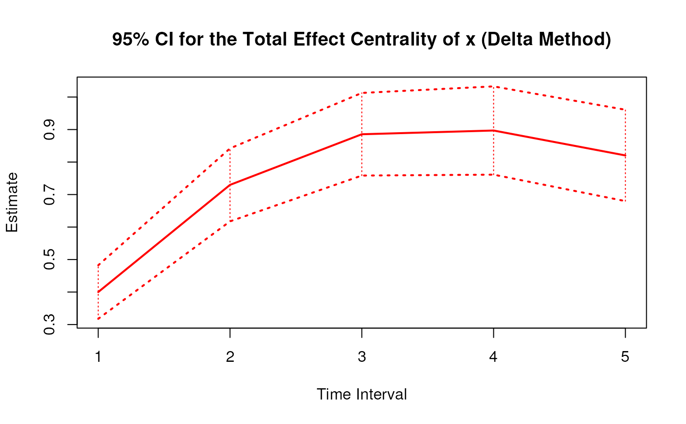
#> 1 x 1 0.4000 0.0485 8.2517 0 0.3050 0.4950
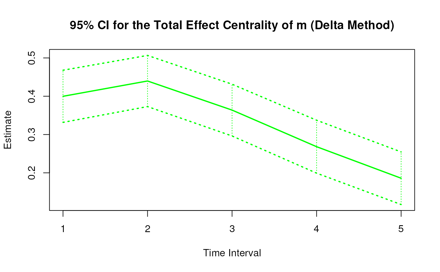
#> 2 m 1 0.3998 0.0411 9.7184 0 0.3192 0.4805
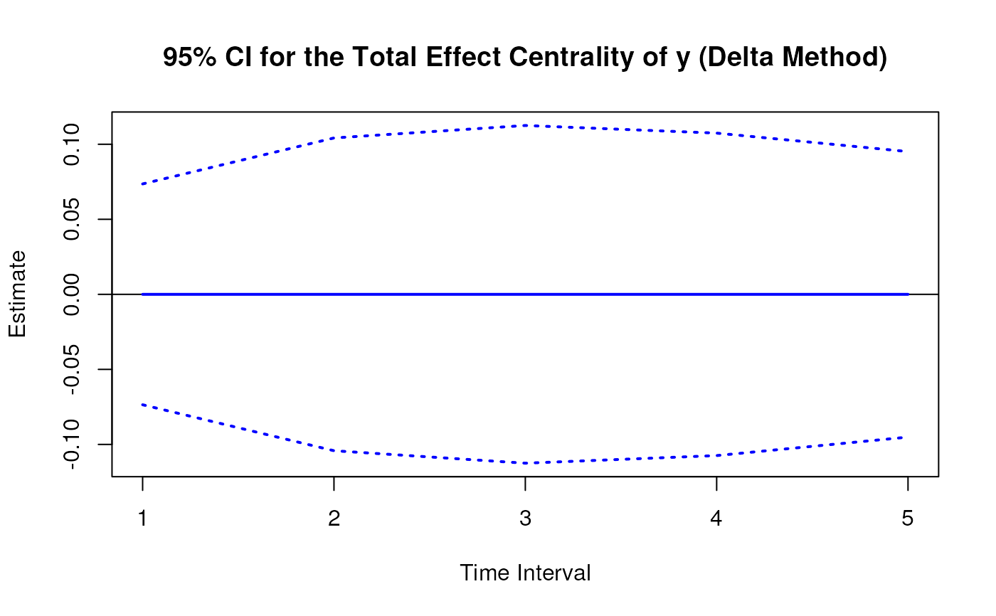
#> 3 y 1 0.0000 0.0650 0.0000 1 -0.1273 0.1273
# Range of time intervals ---------------------------------------------------
delta <- DeltaTotalCentral(
phi = phi,
vcov_phi_vec = vcov_phi_vec,
delta_t = 1:5
)
plot(delta)

 # Methods -------------------------------------------------------------------
# DeltaTotalCentral has a number of methods including
# print, summary, confint, and plot
print(delta)
#> Call:
#> DeltaTotalCentral(phi = phi, vcov_phi_vec = vcov_phi_vec, delta_t = 1:5)
#>
#> Total Effect Centrality
#> variable interval est se z p 2.5% 97.5%
#> 1 x 1 0.4000 0.0485 8.2517 0.0000 0.3050 0.4950
#> 2 m 1 0.3998 0.0411 9.7184 0.0000 0.3192 0.4805
#> 3 y 1 0.0000 0.0650 0.0000 1.0000 -0.1273 0.1273
#> 4 x 2 0.7298 0.0680 10.7288 0.0000 0.5965 0.8631
#> 5 m 2 0.4398 0.0529 8.3137 0.0000 0.3361 0.5435
#> 6 y 2 0.0000 0.0951 0.0000 1.0000 -0.1863 0.1863
#> 7 x 3 0.8855 0.0855 10.3526 0.0000 0.7179 1.0532
#> 8 m 3 0.3638 0.0606 6.0028 0.0000 0.2450 0.4826
#> 9 y 3 0.0000 0.1022 0.0000 1.0000 -0.2004 0.2004
#> 10 x 4 0.8970 0.0999 8.9763 0.0000 0.7012 1.0929
#> 11 m 4 0.2683 0.0659 4.0735 0.0000 0.1392 0.3973
#> 12 y 4 0.0000 0.0961 0.0000 1.0000 -0.1883 0.1883
#> 13 x 5 0.8204 0.1098 7.4745 0.0000 0.6052 1.0355
#> 14 m 5 0.1859 0.0679 2.7368 0.0062 0.0528 0.3191
#> 15 y 5 0.0000 0.0836 0.0000 1.0000 -0.1638 0.1638
summary(delta)
#> Call:
#> DeltaTotalCentral(phi = phi, vcov_phi_vec = vcov_phi_vec, delta_t = 1:5)
#>
#> Total Effect Centrality
#> variable interval est se z p 2.5% 97.5%
#> 1 x 1 0.4000 0.0485 8.2517 0.0000 0.3050 0.4950
#> 2 m 1 0.3998 0.0411 9.7184 0.0000 0.3192 0.4805
#> 3 y 1 0.0000 0.0650 0.0000 1.0000 -0.1273 0.1273
#> 4 x 2 0.7298 0.0680 10.7288 0.0000 0.5965 0.8631
#> 5 m 2 0.4398 0.0529 8.3137 0.0000 0.3361 0.5435
#> 6 y 2 0.0000 0.0951 0.0000 1.0000 -0.1863 0.1863
#> 7 x 3 0.8855 0.0855 10.3526 0.0000 0.7179 1.0532
#> 8 m 3 0.3638 0.0606 6.0028 0.0000 0.2450 0.4826
#> 9 y 3 0.0000 0.1022 0.0000 1.0000 -0.2004 0.2004
#> 10 x 4 0.8970 0.0999 8.9763 0.0000 0.7012 1.0929
#> 11 m 4 0.2683 0.0659 4.0735 0.0000 0.1392 0.3973
#> 12 y 4 0.0000 0.0961 0.0000 1.0000 -0.1883 0.1883
#> 13 x 5 0.8204 0.1098 7.4745 0.0000 0.6052 1.0355
#> 14 m 5 0.1859 0.0679 2.7368 0.0062 0.0528 0.3191
#> 15 y 5 0.0000 0.0836 0.0000 1.0000 -0.1638 0.1638
confint(delta, level = 0.95)
#> variable interval 2.5 % 97.5 %
#> 1 x 1 0.30498791 0.4950036
#> 2 m 1 0.31919849 0.4804728
#> 3 y 1 -0.12734577 0.1273458
#> 4 x 2 0.59646118 0.8630970
#> 5 m 2 0.33612237 0.5434912
#> 6 y 2 -0.18634813 0.1863481
#> 7 x 3 0.71788022 1.0531804
#> 8 m 3 0.24503357 0.4826192
#> 9 y 3 -0.20036471 0.2003647
#> 10 x 4 0.70116982 1.0929020
#> 11 m 4 0.13918690 0.3973317
#> 12 y 4 -0.18831738 0.1883174
#> 13 x 5 0.60524733 1.0354787
#> 14 m 5 0.05277591 0.3190880
#> 15 y 5 -0.16380032 0.1638003
plot(delta)
# Methods -------------------------------------------------------------------
# DeltaTotalCentral has a number of methods including
# print, summary, confint, and plot
print(delta)
#> Call:
#> DeltaTotalCentral(phi = phi, vcov_phi_vec = vcov_phi_vec, delta_t = 1:5)
#>
#> Total Effect Centrality
#> variable interval est se z p 2.5% 97.5%
#> 1 x 1 0.4000 0.0485 8.2517 0.0000 0.3050 0.4950
#> 2 m 1 0.3998 0.0411 9.7184 0.0000 0.3192 0.4805
#> 3 y 1 0.0000 0.0650 0.0000 1.0000 -0.1273 0.1273
#> 4 x 2 0.7298 0.0680 10.7288 0.0000 0.5965 0.8631
#> 5 m 2 0.4398 0.0529 8.3137 0.0000 0.3361 0.5435
#> 6 y 2 0.0000 0.0951 0.0000 1.0000 -0.1863 0.1863
#> 7 x 3 0.8855 0.0855 10.3526 0.0000 0.7179 1.0532
#> 8 m 3 0.3638 0.0606 6.0028 0.0000 0.2450 0.4826
#> 9 y 3 0.0000 0.1022 0.0000 1.0000 -0.2004 0.2004
#> 10 x 4 0.8970 0.0999 8.9763 0.0000 0.7012 1.0929
#> 11 m 4 0.2683 0.0659 4.0735 0.0000 0.1392 0.3973
#> 12 y 4 0.0000 0.0961 0.0000 1.0000 -0.1883 0.1883
#> 13 x 5 0.8204 0.1098 7.4745 0.0000 0.6052 1.0355
#> 14 m 5 0.1859 0.0679 2.7368 0.0062 0.0528 0.3191
#> 15 y 5 0.0000 0.0836 0.0000 1.0000 -0.1638 0.1638
summary(delta)
#> Call:
#> DeltaTotalCentral(phi = phi, vcov_phi_vec = vcov_phi_vec, delta_t = 1:5)
#>
#> Total Effect Centrality
#> variable interval est se z p 2.5% 97.5%
#> 1 x 1 0.4000 0.0485 8.2517 0.0000 0.3050 0.4950
#> 2 m 1 0.3998 0.0411 9.7184 0.0000 0.3192 0.4805
#> 3 y 1 0.0000 0.0650 0.0000 1.0000 -0.1273 0.1273
#> 4 x 2 0.7298 0.0680 10.7288 0.0000 0.5965 0.8631
#> 5 m 2 0.4398 0.0529 8.3137 0.0000 0.3361 0.5435
#> 6 y 2 0.0000 0.0951 0.0000 1.0000 -0.1863 0.1863
#> 7 x 3 0.8855 0.0855 10.3526 0.0000 0.7179 1.0532
#> 8 m 3 0.3638 0.0606 6.0028 0.0000 0.2450 0.4826
#> 9 y 3 0.0000 0.1022 0.0000 1.0000 -0.2004 0.2004
#> 10 x 4 0.8970 0.0999 8.9763 0.0000 0.7012 1.0929
#> 11 m 4 0.2683 0.0659 4.0735 0.0000 0.1392 0.3973
#> 12 y 4 0.0000 0.0961 0.0000 1.0000 -0.1883 0.1883
#> 13 x 5 0.8204 0.1098 7.4745 0.0000 0.6052 1.0355
#> 14 m 5 0.1859 0.0679 2.7368 0.0062 0.0528 0.3191
#> 15 y 5 0.0000 0.0836 0.0000 1.0000 -0.1638 0.1638
confint(delta, level = 0.95)
#> variable interval 2.5 % 97.5 %
#> 1 x 1 0.30498791 0.4950036
#> 2 m 1 0.31919849 0.4804728
#> 3 y 1 -0.12734577 0.1273458
#> 4 x 2 0.59646118 0.8630970
#> 5 m 2 0.33612237 0.5434912
#> 6 y 2 -0.18634813 0.1863481
#> 7 x 3 0.71788022 1.0531804
#> 8 m 3 0.24503357 0.4826192
#> 9 y 3 -0.20036471 0.2003647
#> 10 x 4 0.70116982 1.0929020
#> 11 m 4 0.13918690 0.3973317
#> 12 y 4 -0.18831738 0.1883174
#> 13 x 5 0.60524733 1.0354787
#> 14 m 5 0.05277591 0.3190880
#> 15 y 5 -0.16380032 0.1638003
plot(delta)