Monte Carlo Sampling Distribution of Total, Direct, and Indirect Effects of X on Y Through M Over a Specific Time Interval or a Range of Time Intervals

This function generates a Monte Carlo method sampling distribution of the total, direct and indirect effects of the independent variable $X$ on the dependent variable $Y$ through mediator variables $\mathbf{m}$ over a specific time interval $\Delta t$ or a range of time intervals using the first-order stochastic differential equation model drift matrix $\boldsymbol{\Phi}$.

Usage

MCMed(
  phi,
  vcov_phi_vec,
  delta_t,
  from,
  to,
  med,
  R,
  test_phi = TRUE,
  ncores = NULL,
  seed = NULL
)

Arguments

phi: Numeric matrix. The drift matrix ($\boldsymbol{\Phi}$). phi should have row and column names pertaining to the variables in the system.
vcov_phi_vec: Numeric matrix. The sampling variance-covariance matrix of $\mathrm{vec} \left( \boldsymbol{\Phi} \right)$.
delta_t: Numeric. Time interval ($\Delta t$).
from: Character string. Name of the independent variable $X$ in phi.
to: Character string. Name of the dependent variable $Y$ in phi.
med: Character vector. Name/s of the mediator variable/s in phi.
R: Positive integer. Number of replications.
test_phi: Logical. If test_phi = TRUE, the function tests the stability of the generated drift matrix $\boldsymbol{\Phi}$. If the test returns FALSE, the function generates a new drift matrix $\boldsymbol{\Phi}$ and runs the test recursively until the test returns TRUE.
ncores: Positive integer. Number of cores to use. If ncores = NULL, use a single core. Consider using multiple cores when number of replications R is a large value.
seed: Random seed.

Value

Returns an object of class ctmedmc which is a list with the following elements:

call: Function call.
args: Function arguments.
fun: Function used ("MCMed").
output: A list with length of length(delta_t).

Each element in the output list has the following elements:

est: A vector of total, direct, and indirect effects.
thetahatstar: A matrix of Monte Carlo total, direct, and indirect effects.

Details

See Total(), Direct(), and Indirect() for more details.

Monte Carlo Method

Let $\boldsymbol{\theta}$ be $\mathrm{vec} \left( \boldsymbol{\Phi} \right)$, that is, the elements of the $\boldsymbol{\Phi}$ matrix in vector form sorted column-wise. Let $\hat{\boldsymbol{\theta}}$ be $\mathrm{vec} \left( \hat{\boldsymbol{\Phi}} \right)$. Based on the asymptotic properties of maximum likelihood estimators, we can assume that estimators are normally distributed around the population parameters. $$ \hat{\boldsymbol{\theta}} \sim \mathcal{N} \left( \boldsymbol{\theta}, \mathbb{V} \left( \hat{\boldsymbol{\theta}} \right) \right) $$ Using this distributional assumption, a sampling distribution of $\hat{\boldsymbol{\theta}}$ which we refer to as $\hat{\boldsymbol{\theta}}^{\ast}$ can be generated by replacing the population parameters with sample estimates, that is, $$ \hat{\boldsymbol{\theta}}^{\ast} \sim \mathcal{N} \left( \hat{\boldsymbol{\theta}}, \hat{\mathbb{V}} \left( \hat{\boldsymbol{\theta}} \right) \right) . $$ Let $\mathbf{g} \left( \hat{\boldsymbol{\theta}} \right)$ be a parameter that is a function of the estimated parameters. A sampling distribution of $\mathbf{g} \left( \hat{\boldsymbol{\theta}} \right)$ , which we refer to as $\mathbf{g} \left( \hat{\boldsymbol{\theta}}^{\ast} \right)$ , can be generated by using the simulated estimates to calculate $\mathbf{g}$. The standard deviations of the simulated estimates are the standard errors. Percentiles corresponding to $100 \left( 1 - \alpha \right) \%$ are the confidence intervals.

Linear Stochastic Differential Equation Model

The measurement model is given by $$ \mathbf{y}_{i, t} = \boldsymbol{\nu} + \boldsymbol{\Lambda} \boldsymbol{\eta}_{i, t} + \boldsymbol{\varepsilon}_{i, t}, \quad \mathrm{with} \quad \boldsymbol{\varepsilon}_{i, t} \sim \mathcal{N} \left( \mathbf{0}, \boldsymbol{\Theta} \right) $$ where $\mathbf{y}_{i, t}$, $\boldsymbol{\eta}_{i, t}$, and $\boldsymbol{\varepsilon}_{i, t}$ are random variables and $\boldsymbol{\nu}$, $\boldsymbol{\Lambda}$, and $\boldsymbol{\Theta}$ are model parameters. $\mathbf{y}_{i, t}$ represents a vector of observed random variables, $\boldsymbol{\eta}_{i, t}$ a vector of latent random variables, and $\boldsymbol{\varepsilon}_{i, t}$ a vector of random measurement errors, at time $t$ and individual $i$. $\boldsymbol{\nu}$ denotes a vector of intercepts, $\boldsymbol{\Lambda}$ a matrix of factor loadings, and $\boldsymbol{\Theta}$ the covariance matrix of $\boldsymbol{\varepsilon}$.

An alternative representation of the measurement error is given by $$ \boldsymbol{\varepsilon}_{i, t} = \boldsymbol{\Theta}^{\frac{1}{2}} \mathbf{z}_{i, t}, \quad \mathrm{with} \quad \mathbf{z}_{i, t} \sim \mathcal{N} \left( \mathbf{0}, \mathbf{I} \right) $$ where $\mathbf{z}_{i, t}$ is a vector of independent standard normal random variables and $ \left( \boldsymbol{\Theta}^{\frac{1}{2}} \right) \left( \boldsymbol{\Theta}^{\frac{1}{2}} \right)^{\prime} = \boldsymbol{\Theta} . $

The dynamic structure is given by $$ \mathrm{d} \boldsymbol{\eta}_{i, t} = \left( \boldsymbol{\iota} + \boldsymbol{\Phi} \boldsymbol{\eta}_{i, t} \right) \mathrm{d}t + \boldsymbol{\Sigma}^{\frac{1}{2}} \mathrm{d} \mathbf{W}_{i, t} $$ where $\boldsymbol{\iota}$ is a term which is unobserved and constant over time, $\boldsymbol{\Phi}$ is the drift matrix which represents the rate of change of the solution in the absence of any random fluctuations, $\boldsymbol{\Sigma}$ is the matrix of volatility or randomness in the process, and $\mathrm{d}\boldsymbol{W}$ is a Wiener process or Brownian motion, which represents random fluctuations.

References

Bollen, K. A. (1987). Total, direct, and indirect effects in structural equation models. Sociological Methodology, 17, 37. doi:10.2307/271028

Deboeck, P. R., & Preacher, K. J. (2015). No need to be discrete: A method for continuous time mediation analysis. Structural Equation Modeling: A Multidisciplinary Journal, 23 (1), 61–75. doi:10.1080/10705511.2014.973960

Ryan, O., & Hamaker, E. L. (2021). Time to intervene: A continuous-time approach to network analysis and centrality. Psychometrika, 87 (1), 214–252. doi:10.1007/s11336-021-09767-0

Author

Ivan Jacob Agaloos Pesigan

Examples

set.seed(42)
phi <- matrix(
  data = c(
    -0.357, 0.771, -0.450,
    0.0, -0.511, 0.729,
    0, 0, -0.693
  ),
  nrow = 3
)
colnames(phi) <- rownames(phi) <- c("x", "m", "y")
vcov_phi_vec <- matrix(
  data = c(
    0.002704274, -0.001475275, 0.000949122,
    -0.001619422, 0.000885122, -0.000569404,
    0.00085493, -0.000465824, 0.000297815,
    -0.001475275, 0.004428442, -0.002642303,
    0.000980573, -0.00271817, 0.001618805,
    -0.000586921, 0.001478421, -0.000871547,
    0.000949122, -0.002642303, 0.006402668,
    -0.000697798, 0.001813471, -0.004043138,
    0.000463086, -0.001120949, 0.002271711,
    -0.001619422, 0.000980573, -0.000697798,
    0.002079286, -0.001152501, 0.000753,
    -0.001528701, 0.000820587, -0.000517524,
    0.000885122, -0.00271817, 0.001813471,
    -0.001152501, 0.00342605, -0.002075005,
    0.000899165, -0.002532849, 0.001475579,
    -0.000569404, 0.001618805, -0.004043138,
    0.000753, -0.002075005, 0.004984032,
    -0.000622255, 0.001634917, -0.003705661,
    0.00085493, -0.000586921, 0.000463086,
    -0.001528701, 0.000899165, -0.000622255,
    0.002060076, -0.001096684, 0.000686386,
    -0.000465824, 0.001478421, -0.001120949,
    0.000820587, -0.002532849, 0.001634917,
    -0.001096684, 0.003328692, -0.001926088,
    0.000297815, -0.000871547, 0.002271711,
    -0.000517524, 0.001475579, -0.003705661,
    0.000686386, -0.001926088, 0.004726235
  ),
  nrow = 9
)

# Specific time interval ----------------------------------------------------
MCMed(
  phi = phi,
  vcov_phi_vec = vcov_phi_vec,
  delta_t = 1,
  from = "x",
  to = "y",
  med = "m",
  R = 100L # use a large value for R in actual research
)
#> 
#> Total, Direct, and Indirect Effects
#> 
#> $`1`
#>          interval     est     se   R    2.5%   97.5%
#> total           1 -0.1000 0.0342 100 -0.1666 -0.0440
#> direct          1 -0.2675 0.0440 100 -0.3567 -0.1863
#> indirect        1  0.1674 0.0201 100  0.1273  0.2006
#> 

# Range of time intervals ---------------------------------------------------
mc <- MCMed(
  phi = phi,
  vcov_phi_vec = vcov_phi_vec,
  delta_t = 1:5,
  from = "x",
  to = "y",
  med = "m",
  R = 100L # use a large value for R in actual research
)
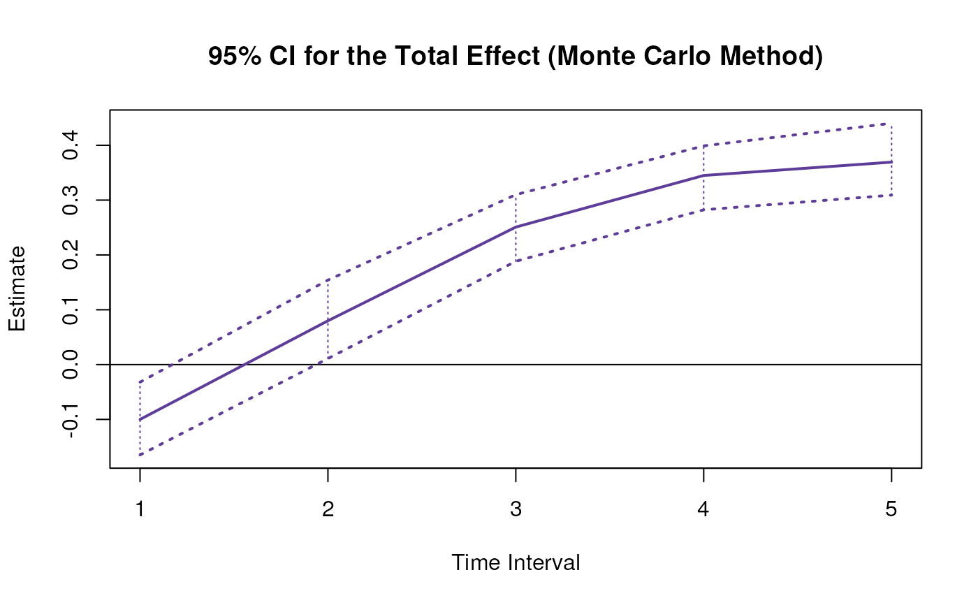
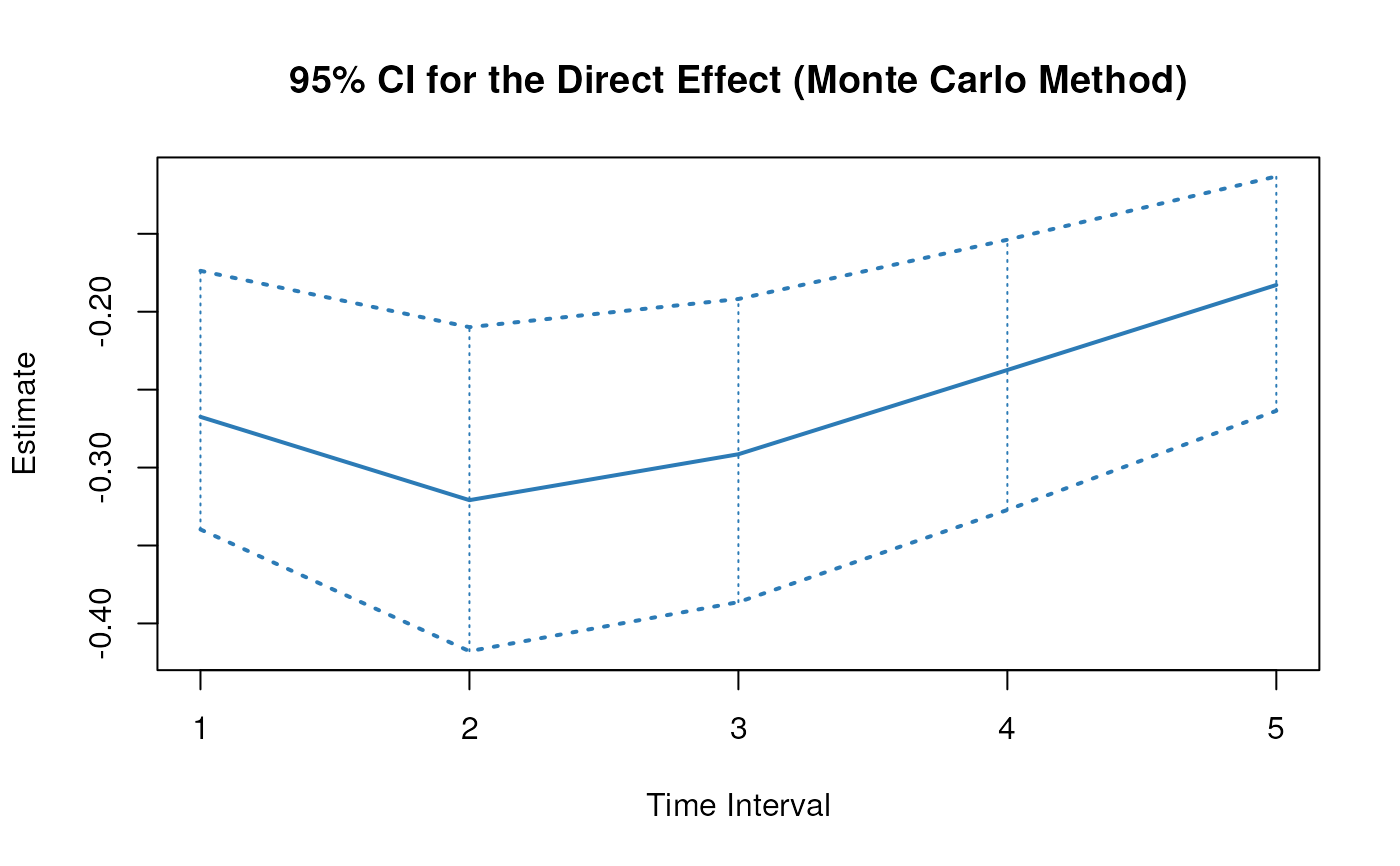
plot(mc)




# Methods -------------------------------------------------------------------
# MCMed has a number of methods including
# print, summary, confint, and plot
print(mc)
#> 
#> Total, Direct, and Indirect Effects
#> 
#> $`1`
#>          interval     est     se   R    2.5%   97.5%
#> total           1 -0.1000 0.0340 100 -0.1648 -0.0320
#> direct          1 -0.2675 0.0471 100 -0.3397 -0.1738
#> indirect        1  0.1674 0.0201 100  0.1239  0.1982
#> 
#> $`2`
#>          interval     est     se   R    2.5%   97.5%
#> total           2  0.0799 0.0352 100  0.0110  0.1542
#> direct          2 -0.3209 0.0555 100 -0.4178 -0.2099
#> indirect        2  0.4008 0.0413 100  0.3090  0.4663
#> 
#> $`3`
#>          interval     est     se   R    2.5%   97.5%
#> total           3  0.2508 0.0337 100  0.1884  0.3100
#> direct          3 -0.2914 0.0524 100 -0.3863 -0.1918
#> indirect        3  0.5423 0.0523 100  0.4351  0.6286
#> 
#> $`4`
#>          interval     est     se   R    2.5%   97.5%
#> total           4  0.3449 0.0324 100  0.2823  0.3989
#> direct          4 -0.2374 0.0464 100 -0.3272 -0.1538
#> indirect        4  0.5823 0.0575 100  0.4668  0.6888
#> 
#> $`5`
#>          interval     est     se   R    2.5%   97.5%
#> total           5  0.3693 0.0325 100  0.3091  0.4402
#> direct          5 -0.1828 0.0402 100 -0.2636 -0.1132
#> indirect        5  0.5521 0.0594 100  0.4404  0.6682
#> 
summary(mc)
#>      effect interval        est         se   R        2.5%      97.5%
#> 1     total        1 -0.1000384 0.03395899 100 -0.16476025 -0.0320114
#> 2    direct        1 -0.2674539 0.04709743 100 -0.33969758 -0.1737522
#> 3  indirect        1  0.1674155 0.02007626 100  0.12388402  0.1982442
#> 4     total        2  0.0799008 0.03520320 100  0.01098553  0.1541882
#> 5    direct        2 -0.3209035 0.05552653 100 -0.41779752 -0.2098965
#> 6  indirect        2  0.4008043 0.04125368 100  0.30898862  0.4662702
#> 7     total        3  0.2508138 0.03368900 100  0.18841270  0.3099660
#> 8    direct        3 -0.2914426 0.05239901 100 -0.38632534 -0.1918376
#> 9  indirect        3  0.5422564 0.05233930 100  0.43511469  0.6285914
#> 10    total        4  0.3449279 0.03244313 100  0.28231133  0.3989232
#> 11   direct        4 -0.2373900 0.04644744 100 -0.32719487 -0.1538166
#> 12 indirect        4  0.5823179 0.05746986 100  0.46682812  0.6888180
#> 13    total        5  0.3692538 0.03254938 100  0.30907920  0.4401860
#> 14   direct        5 -0.1828447 0.04019984 100 -0.26357998 -0.1131929
#> 15 indirect        5  0.5520985 0.05939646 100  0.44035670  0.6682153
confint(mc, level = 0.95)
#>      effect interval       2.5 %     97.5 %
#> 1     total        1 -0.16476025 -0.0320114
#> 2    direct        1 -0.33969758 -0.1737522
#> 3  indirect        1  0.12388402  0.1982442
#> 4     total        2  0.01098553  0.1541882
#> 5    direct        2 -0.41779752 -0.2098965
#> 6  indirect        2  0.30898862  0.4662702
#> 7     total        3  0.18841270  0.3099660
#> 8    direct        3 -0.38632534 -0.1918376
#> 9  indirect        3  0.43511469  0.6285914
#> 10    total        4  0.28231133  0.3989232
#> 11   direct        4 -0.32719487 -0.1538166
#> 12 indirect        4  0.46682812  0.6888180
#> 13    total        5  0.30907920  0.4401860
#> 14   direct        5 -0.26357998 -0.1131929
#> 15 indirect        5  0.44035670  0.6682153