Total, Direct, and Indirect Effects of X on Y Through M Over a Specific Time Interval or a Range of Time Intervals

This function computes the total, direct, and indirect effects of the independent variable $X$ on the dependent variable $Y$ through mediator variables $\mathbf{m}$ over a specific time interval $\Delta t$ or a range of time intervals using the first-order stochastic differential equation model's drift matrix $\boldsymbol{\Phi}$.

Usage

Med(phi, delta_t, from, to, med)

Arguments

phi: Numeric matrix. The drift matrix ($\boldsymbol{\Phi}$). phi should have row and column names pertaining to the variables in the system.
delta_t: Vector of positive numbers. Time interval ($\Delta t$).
from: Character string. Name of the independent variable $X$ in phi.
to: Character string. Name of the dependent variable $Y$ in phi.
med: Character vector. Name/s of the mediator variable/s in phi.

Value

Returns an object of class ctmedmed which is a list with the following elements:

call: Function call.
args: Function arguments.
fun: Function used ("Med").
output: A matrix of total, direct, and indirect effects.

Details

See Total(), Direct(), and Indirect() for more details.

Linear Stochastic Differential Equation Model

The measurement model is given by $$ \mathbf{y}_{i, t} = \boldsymbol{\nu} + \boldsymbol{\Lambda} \boldsymbol{\eta}_{i, t} + \boldsymbol{\varepsilon}_{i, t}, \quad \mathrm{with} \quad \boldsymbol{\varepsilon}_{i, t} \sim \mathcal{N} \left( \mathbf{0}, \boldsymbol{\Theta} \right) $$ where $\mathbf{y}_{i, t}$, $\boldsymbol{\eta}_{i, t}$, and $\boldsymbol{\varepsilon}_{i, t}$ are random variables and $\boldsymbol{\nu}$, $\boldsymbol{\Lambda}$, and $\boldsymbol{\Theta}$ are model parameters. $\mathbf{y}_{i, t}$ represents a vector of observed random variables, $\boldsymbol{\eta}_{i, t}$ a vector of latent random variables, and $\boldsymbol{\varepsilon}_{i, t}$ a vector of random measurement errors, at time $t$ and individual $i$. $\boldsymbol{\nu}$ denotes a vector of intercepts, $\boldsymbol{\Lambda}$ a matrix of factor loadings, and $\boldsymbol{\Theta}$ the covariance matrix of $\boldsymbol{\varepsilon}$.

An alternative representation of the measurement error is given by $$ \boldsymbol{\varepsilon}_{i, t} = \boldsymbol{\Theta}^{\frac{1}{2}} \mathbf{z}_{i, t}, \quad \mathrm{with} \quad \mathbf{z}_{i, t} \sim \mathcal{N} \left( \mathbf{0}, \mathbf{I} \right) $$ where $\mathbf{z}_{i, t}$ is a vector of independent standard normal random variables and $ \left( \boldsymbol{\Theta}^{\frac{1}{2}} \right) \left( \boldsymbol{\Theta}^{\frac{1}{2}} \right)^{\prime} = \boldsymbol{\Theta} . $

The dynamic structure is given by $$ \mathrm{d} \boldsymbol{\eta}_{i, t} = \left( \boldsymbol{\iota} + \boldsymbol{\Phi} \boldsymbol{\eta}_{i, t} \right) \mathrm{d}t + \boldsymbol{\Sigma}^{\frac{1}{2}} \mathrm{d} \mathbf{W}_{i, t} $$ where $\boldsymbol{\iota}$ is a term which is unobserved and constant over time, $\boldsymbol{\Phi}$ is the drift matrix which represents the rate of change of the solution in the absence of any random fluctuations, $\boldsymbol{\Sigma}$ is the matrix of volatility or randomness in the process, and $\mathrm{d}\boldsymbol{W}$ is a Wiener process or Brownian motion, which represents random fluctuations.

References

Bollen, K. A. (1987). Total, direct, and indirect effects in structural equation models. Sociological Methodology, 17, 37. doi:10.2307/271028

Deboeck, P. R., & Preacher, K. J. (2015). No need to be discrete: A method for continuous time mediation analysis. Structural Equation Modeling: A Multidisciplinary Journal, 23 (1), 61–75. doi:10.1080/10705511.2014.973960

Ryan, O., & Hamaker, E. L. (2021). Time to intervene: A continuous-time approach to network analysis and centrality. Psychometrika, 87 (1), 214–252. doi:10.1007/s11336-021-09767-0

Author

Ivan Jacob Agaloos Pesigan

Examples

phi <- matrix(
  data = c(
    -0.357, 0.771, -0.450,
    0.0, -0.511, 0.729,
    0, 0, -0.693
  ),
  nrow = 3
)
colnames(phi) <- rownames(phi) <- c("x", "m", "y")

# Specific time interval ----------------------------------------------------
Med(
  phi = phi,
  delta_t = 1,
  from = "x",
  to = "y",
  med = "m"
)
#> 
#> Total, Direct, and Indirect Effects
#> 
#>      interval total  direct indirect
#> [1,]        1  -0.1 -0.2675   0.1674

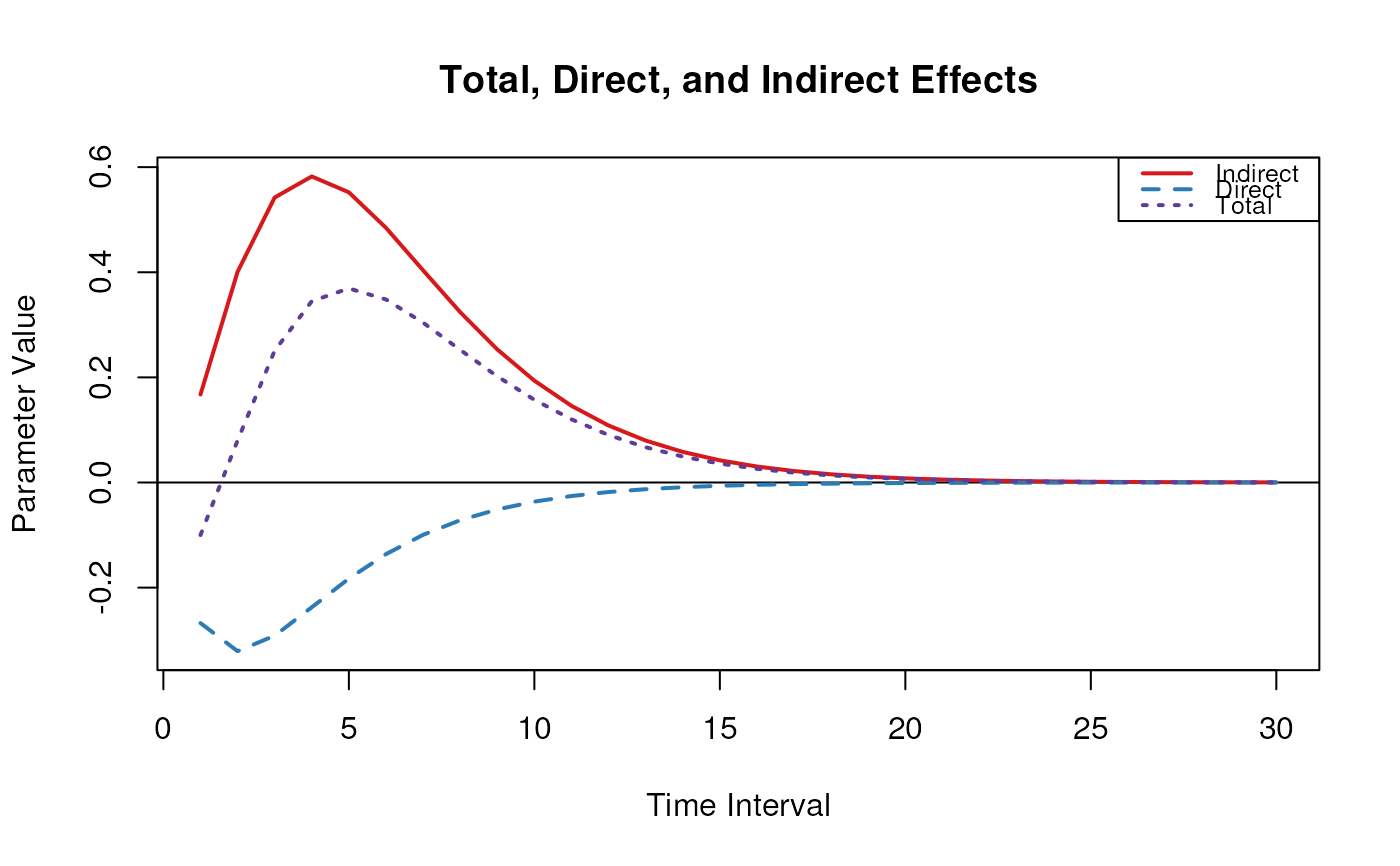
# Range of time intervals ---------------------------------------------------
med <- Med(
  phi = phi,
  delta_t = 1:30,
  from = "x",
  to = "y",
  med = "m"
)
plot(med)


# Methods -------------------------------------------------------------------
# Med has a number of methods including
# print, summary, and plot
med <- Med(
  phi = phi,
  delta_t = 1:5,
  from = "x",
  to = "y",
  med = "m"
)
print(med)
#> 
#> Total, Direct, and Indirect Effects
#> 
#>      interval   total  direct indirect
#> [1,]        1 -0.1000 -0.2675   0.1674
#> [2,]        2  0.0799 -0.3209   0.4008
#> [3,]        3  0.2508 -0.2914   0.5423
#> [4,]        4  0.3449 -0.2374   0.5823
#> [5,]        5  0.3693 -0.1828   0.5521
summary(med)
#>      interval   total  direct indirect
#> [1,]        1 -0.1000 -0.2675   0.1674
#> [2,]        2  0.0799 -0.3209   0.4008
#> [3,]        3  0.2508 -0.2914   0.5423
#> [4,]        4  0.3449 -0.2374   0.5823
#> [5,]        5  0.3693 -0.1828   0.5521
plot(med)