Standardized Total, Direct, and Indirect Effects of X on Y Through M Over a Specific Time Interval or a Range of Time Intervals
Source:R/cTMed-med-std.R
MedStd.RdThis function computes the standardized total, direct, and indirect effects of the independent variable \(X\) on the dependent variable \(Y\) through mediator variables \(\mathbf{m}\) over a specific time interval \(\Delta t\) or a range of time intervals using the first-order stochastic differential equation model's drift matrix \(\boldsymbol{\Phi}\) and process noise covariance matrix \(\boldsymbol{\Sigma}\).
Arguments
- phi
Numeric matrix. The drift matrix (\(\boldsymbol{\Phi}\)).
phishould have row and column names pertaining to the variables in the system.- sigma
Numeric matrix. The process noise covariance matrix (\(\boldsymbol{\Sigma}\)).
- delta_t
Numeric. Time interval (\(\Delta t\)).
- from
Character string. Name of the independent variable \(X\) in
phi.- to
Character string. Name of the dependent variable \(Y\) in
phi.- med
Character vector. Name/s of the mediator variable/s in
phi.- tol
Numeric. Smallest possible time interval to allow.
Value
Returns an object
of class ctmedmed which is a list with the following elements:
- call
Function call.
- args
Function arguments.
- fun
Function used ("MedStd").
- output
A standardized matrix of total, direct, and indirect effects.
Details
See TotalStd(),
DirectStd(), and
IndirectStd() for more details.
References
Bollen, K. A. (1987). Total, direct, and indirect effects in structural equation models. Sociological Methodology, 17, 37. doi:10.2307/271028
Deboeck, P. R., & Preacher, K. J. (2015). No need to be discrete: A method for continuous time mediation analysis. Structural Equation Modeling: A Multidisciplinary Journal, 23 (1), 61-75. doi:10.1080/10705511.2014.973960
Pesigan, I. J. A., Russell, M. A., & Chow, S.-M. (2025). Inferences and effect sizes for direct, indirect, and total effects in continuous-time mediation models. Psychological Methods. doi:10.1037/met0000779
Ryan, O., & Hamaker, E. L. (2021). Time to intervene: A continuous-time approach to network analysis and centrality. Psychometrika, 87 (1), 214-252. doi:10.1007/s11336-021-09767-0
See also
Other Continuous-Time Mediation Functions:
BootBeta(),
BootBetaStd(),
BootDirectCentral(),
BootDirectCentralStd(),
BootIndirectCentral(),
BootIndirectCentralStd(),
BootMed(),
BootMedStd(),
BootTotalCentral(),
BootTotalCentralStd(),
DeltaBeta(),
DeltaBetaStd(),
DeltaDirectCentral(),
DeltaDirectCentralStd(),
DeltaIndirectCentral(),
DeltaMed(),
DeltaMedStd(),
DeltaTotalCentral(),
DeltaTotalCentralStd(),
Direct(),
DirectCentral(),
DirectCentralStd(),
DirectStd(),
Indirect(),
IndirectCentral(),
IndirectCentralStd(),
IndirectStd(),
MCBeta(),
MCBetaStd(),
MCDirectCentral(),
MCDirectCentralStd(),
MCIndirectCentral(),
MCIndirectCentralStd(),
MCMed(),
MCMedStd(),
MCPhi(),
MCPhiSigma(),
MCTotalCentral(),
MCTotalCentralStd(),
Med(),
PosteriorBeta(),
PosteriorBetaStd(),
PosteriorDirectCentral(),
PosteriorDirectCentralStd(),
PosteriorIndirectCentral(),
PosteriorIndirectCentralStd(),
PosteriorMed(),
PosteriorMedStd(),
PosteriorTotalCentral(),
PosteriorTotalCentralStd(),
Total(),
TotalCentral(),
TotalCentralStd(),
TotalStd(),
Trajectory()
Examples
phi <- matrix(
data = c(
-0.357, 0.771, -0.450,
0.0, -0.511, 0.729,
0, 0, -0.693
),
nrow = 3
)
colnames(phi) <- rownames(phi) <- c("x", "m", "y")
sigma <- matrix(
data = c(
0.24455556, 0.02201587, -0.05004762,
0.02201587, 0.07067800, 0.01539456,
-0.05004762, 0.01539456, 0.07553061
),
nrow = 3
)
# Specific time interval ----------------------------------------------------
MedStd(
phi = phi,
sigma = sigma,
delta_t = 1,
from = "x",
to = "y",
med = "m"
)
#> Call:
#> MedStd(phi = phi, sigma = sigma, delta_t = 1, from = "x", to = "y",
#> med = "m")
#>
#> Total, Direct, and Indirect Effects
#>
#> interval total direct indirect
#> [1,] 1 -0.1069 -0.2858 0.1789
# Range of time intervals ---------------------------------------------------
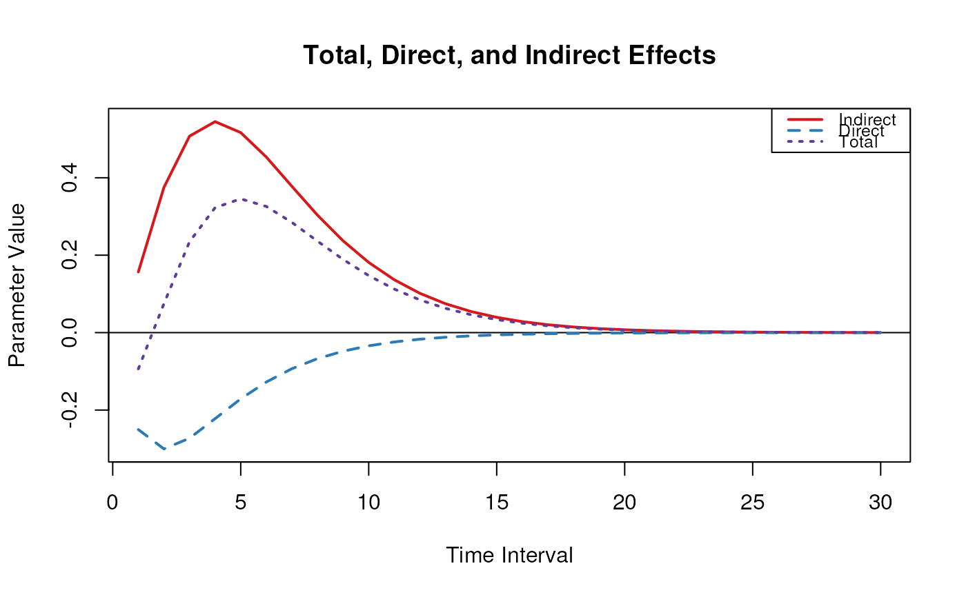
med <- MedStd(
phi = phi,
sigma = sigma,
delta_t = 1:30,
from = "x",
to = "y",
med = "m"
)
plot(med)
 # Methods -------------------------------------------------------------------
# MedStd has a number of methods including
# print, summary, and plot
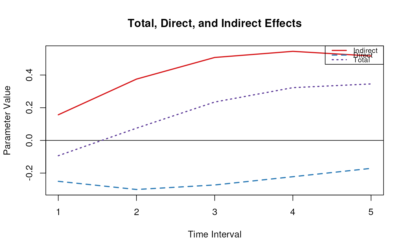
med <- MedStd(
phi = phi,
sigma = sigma,
delta_t = 1:5,
from = "x",
to = "y",
med = "m"
)
print(med)
#> Call:
#> MedStd(phi = phi, sigma = sigma, delta_t = 1:5, from = "x", to = "y",
#> med = "m")
#>
#> Total, Direct, and Indirect Effects
#>
#> interval total direct indirect
#> [1,] 1 -0.1069 -0.2858 0.1789
#> [2,] 2 0.0854 -0.3429 0.4283
#> [3,] 3 0.2680 -0.3114 0.5794
#> [4,] 4 0.3686 -0.2537 0.6222
#> [5,] 5 0.3946 -0.1954 0.5899
summary(med)
#> Call:
#> MedStd(phi = phi, sigma = sigma, delta_t = 1:5, from = "x", to = "y",
#> med = "m")
#>
#> Total, Direct, and Indirect Effects
#>
#> interval total direct indirect
#> [1,] 1 -0.1069 -0.2858 0.1789
#> [2,] 2 0.0854 -0.3429 0.4283
#> [3,] 3 0.2680 -0.3114 0.5794
#> [4,] 4 0.3686 -0.2537 0.6222
#> [5,] 5 0.3946 -0.1954 0.5899
plot(med)
# Methods -------------------------------------------------------------------
# MedStd has a number of methods including
# print, summary, and plot
med <- MedStd(
phi = phi,
sigma = sigma,
delta_t = 1:5,
from = "x",
to = "y",
med = "m"
)
print(med)
#> Call:
#> MedStd(phi = phi, sigma = sigma, delta_t = 1:5, from = "x", to = "y",
#> med = "m")
#>
#> Total, Direct, and Indirect Effects
#>
#> interval total direct indirect
#> [1,] 1 -0.1069 -0.2858 0.1789
#> [2,] 2 0.0854 -0.3429 0.4283
#> [3,] 3 0.2680 -0.3114 0.5794
#> [4,] 4 0.3686 -0.2537 0.6222
#> [5,] 5 0.3946 -0.1954 0.5899
summary(med)
#> Call:
#> MedStd(phi = phi, sigma = sigma, delta_t = 1:5, from = "x", to = "y",
#> med = "m")
#>
#> Total, Direct, and Indirect Effects
#>
#> interval total direct indirect
#> [1,] 1 -0.1069 -0.2858 0.1789
#> [2,] 2 0.0854 -0.3429 0.4283
#> [3,] 3 0.2680 -0.3114 0.5794
#> [4,] 4 0.3686 -0.2537 0.6222
#> [5,] 5 0.3946 -0.1954 0.5899
plot(med)