Delta Method Sampling Variance-Covariance Matrix for the Elements of the Standardized Matrix of Lagged Coefficients Over a Specific Time Interval or a Range of Time Intervals
Source:R/cTMed-delta-beta-std.R
DeltaBetaStd.RdThis function computes the delta method sampling variance-covariance matrix for the elements of the standardized matrix of lagged coefficients \(\boldsymbol{\beta}\) over a specific time interval \(\Delta t\) or a range of time intervals using the first-order stochastic differential equation model's drift matrix \(\boldsymbol{\Phi}\) and process noise covariance matrix \(\boldsymbol{\Sigma}\).
Usage
DeltaBetaStd(
  phi,
  sigma,
  vcov_theta,
  delta_t,
  sigma_diag = FALSE,
  ncores = NULL,
  tol = 0.001
)
Arguments
- phi
Numeric matrix. The drift matrix (\(\boldsymbol{\Phi}\)).
phishould have row and column names pertaining to the variables in the system.- sigma
Numeric matrix. The process noise covariance matrix (\(\boldsymbol{\Sigma}\)).
- vcov_theta
Numeric matrix. The sampling variance-covariance matrix of \(\mathrm{vec} \left( \boldsymbol{\Phi} \right)\) and \(\mathrm{vech} \left( \boldsymbol{\Sigma} \right)\)
- delta_t
Numeric. Time interval (\(\Delta t\)).
- sigma_diag
Logical. If
sigma_diag = TRUE, treat \(\boldsymbol{\Sigma}\) as a diagonal matrix.- ncores
Positive integer. Number of cores to use. If
ncores = NULL, use a single core. Consider using multiple cores when number of replicationsRis a large value.- tol
Numeric. Smallest possible time interval to allow.
Value
Returns an object
of class ctmeddelta which is a list with the following elements:
- call
Function call.
- args
Function arguments.
- fun
Function used ("DeltaBetaStd").
- output
A list of length
length(delta_t).
Each element in the output list has the following elements:
- delta_t
Time interval.
- jacobian
Jacobian matrix.
- est
Estimated elements of the standardized matrix of lagged coefficients.
- vcov
Sampling variance-covariance matrix of estimated elements of the standardized matrix of lagged coefficients.
Details
See TotalStd().
Delta Method
Let \(\boldsymbol{\theta}\) be a vector that combines \(\mathrm{vec} \left( \boldsymbol{\Phi} \right)\), that is, the elements of the \(\boldsymbol{\Phi}\) matrix in vector form sorted column-wise and \(\mathrm{vech} \left( \boldsymbol{\Sigma} \right)\), that is, the unique elements of the \(\boldsymbol{\Sigma}\) matrix in vector form sorted column-wise. Let \(\hat{\boldsymbol{\theta}}\) be a vector that combines \(\mathrm{vec} \left( \hat{\boldsymbol{\Phi}} \right)\) and \(\mathrm{vech} \left( \hat{\boldsymbol{\Sigma}} \right)\). By the multivariate central limit theory, the function \(\mathbf{g}\) using \(\hat{\boldsymbol{\theta}}\) as input can be expressed as:
$$ \sqrt{n} \left( \mathbf{g} \left( \hat{\boldsymbol{\theta}} \right) - \mathbf{g} \left( \boldsymbol{\theta} \right) \right) \xrightarrow[]{ \mathrm{D} } \mathcal{N} \left( 0, \mathbf{J} \boldsymbol{\Gamma} \mathbf{J}^{\prime} \right) $$
where \(\mathbf{J}\) is the matrix of first-order derivatives of the function \(\mathbf{g}\) with respect to the elements of \(\boldsymbol{\theta}\) and \(\boldsymbol{\Gamma}\) is the asymptotic variance-covariance matrix of \(\hat{\boldsymbol{\theta}}\).
From the former, we can derive the distribution of \(\mathbf{g} \left( \hat{\boldsymbol{\theta}} \right)\) as follows:
$$ \mathbf{g} \left( \hat{\boldsymbol{\theta}} \right) \approx \mathcal{N} \left( \mathbf{g} \left( \boldsymbol{\theta} \right) , n^{-1} \mathbf{J} \boldsymbol{\Gamma} \mathbf{J}^{\prime} \right) $$
The uncertainty associated with the estimator \(\mathbf{g} \left( \hat{\boldsymbol{\theta}} \right)\) is, therefore, given by \(n^{-1} \mathbf{J} \boldsymbol{\Gamma} \mathbf{J}^{\prime}\) . When \(\boldsymbol{\Gamma}\) is unknown, by substitution, we can use the estimated sampling variance-covariance matrix of \(\hat{\boldsymbol{\theta}}\), that is, \(\hat{\mathbb{V}} \left( \hat{\boldsymbol{\theta}} \right)\) for \(n^{-1} \boldsymbol{\Gamma}\). Therefore, the sampling variance-covariance matrix of \(\mathbf{g} \left( \hat{\boldsymbol{\theta}} \right)\) is given by
$$ \mathbf{g} \left( \hat{\boldsymbol{\theta}} \right) \approx \mathcal{N} \left( \mathbf{g} \left( \boldsymbol{\theta} \right) , \mathbf{J} \hat{\mathbb{V}} \left( \hat{\boldsymbol{\theta}} \right) \mathbf{J}^{\prime} \right) . $$
References
Bollen, K. A. (1987). Total, direct, and indirect effects in structural equation models. Sociological Methodology, 17, 37. doi:10.2307/271028
Deboeck, P. R., & Preacher, K. J. (2015). No need to be discrete: A method for continuous time mediation analysis. Structural Equation Modeling: A Multidisciplinary Journal, 23 (1), 61-75. doi:10.1080/10705511.2014.973960
Pesigan, I. J. A., Russell, M. A., & Chow, S.-M. (2025). Inferences and effect sizes for direct, indirect, and total effects in continuous-time mediation models. Psychological Methods. doi:10.1037/met0000779
Ryan, O., & Hamaker, E. L. (2021). Time to intervene: A continuous-time approach to network analysis and centrality. Psychometrika, 87 (1), 214-252. doi:10.1007/s11336-021-09767-0
See also
Other Continuous-Time Mediation Functions:
BootBeta(),
BootBetaStd(),
BootDirectCentral(),
BootDirectCentralStd(),
BootIndirectCentral(),
BootIndirectCentralStd(),
BootMed(),
BootMedStd(),
BootTotalCentral(),
BootTotalCentralStd(),
DeltaBeta(),
DeltaDirectCentral(),
DeltaDirectCentralStd(),
DeltaIndirectCentral(),
DeltaMed(),
DeltaMedStd(),
DeltaTotalCentral(),
DeltaTotalCentralStd(),
Direct(),
DirectCentral(),
DirectCentralStd(),
DirectStd(),
Indirect(),
IndirectCentral(),
IndirectCentralStd(),
IndirectStd(),
MCBeta(),
MCBetaStd(),
MCDirectCentral(),
MCDirectCentralStd(),
MCIndirectCentral(),
MCIndirectCentralStd(),
MCMed(),
MCMedStd(),
MCPhi(),
MCPhiSigma(),
MCTotalCentral(),
MCTotalCentralStd(),
Med(),
MedStd(),
PosteriorBeta(),
PosteriorBetaStd(),
PosteriorDirectCentral(),
PosteriorDirectCentralStd(),
PosteriorIndirectCentral(),
PosteriorIndirectCentralStd(),
PosteriorMed(),
PosteriorMedStd(),
PosteriorTotalCentral(),
PosteriorTotalCentralStd(),
Total(),
TotalCentral(),
TotalCentralStd(),
TotalStd(),
Trajectory()
Examples
phi <- matrix(
data = c(
-0.357, 0.771, -0.450,
0.0, -0.511, 0.729,
0, 0, -0.693
),
nrow = 3
)
colnames(phi) <- rownames(phi) <- c("x", "m", "y")
sigma <- matrix(
data = c(
0.24455556, 0.02201587, -0.05004762,
0.02201587, 0.07067800, 0.01539456,
-0.05004762, 0.01539456, 0.07553061
),
nrow = 3
)
vcov_theta <- matrix(
data = c(
0.00843, 0.00040, -0.00151, -0.00600, -0.00033,
0.00110, 0.00324, 0.00020, -0.00061, -0.00115,
0.00011, 0.00015, 0.00001, -0.00002, -0.00001,
0.00040, 0.00374, 0.00016, -0.00022, -0.00273,
-0.00016, 0.00009, 0.00150, 0.00012, -0.00010,
-0.00026, 0.00002, 0.00012, 0.00004, -0.00001,
-0.00151, 0.00016, 0.00389, 0.00103, -0.00007,
-0.00283, -0.00050, 0.00000, 0.00156, 0.00021,
-0.00005, -0.00031, 0.00001, 0.00007, 0.00006,
-0.00600, -0.00022, 0.00103, 0.00644, 0.00031,
-0.00119, -0.00374, -0.00021, 0.00070, 0.00064,
-0.00015, -0.00005, 0.00000, 0.00003, -0.00001,
-0.00033, -0.00273, -0.00007, 0.00031, 0.00287,
0.00013, -0.00014, -0.00170, -0.00012, 0.00006,
0.00014, -0.00001, -0.00015, 0.00000, 0.00001,
0.00110, -0.00016, -0.00283, -0.00119, 0.00013,
0.00297, 0.00063, -0.00004, -0.00177, -0.00013,
0.00005, 0.00017, -0.00002, -0.00008, 0.00001,
0.00324, 0.00009, -0.00050, -0.00374, -0.00014,
0.00063, 0.00495, 0.00024, -0.00093, -0.00020,
0.00006, -0.00010, 0.00000, -0.00001, 0.00004,
0.00020, 0.00150, 0.00000, -0.00021, -0.00170,
-0.00004, 0.00024, 0.00214, 0.00012, -0.00002,
-0.00004, 0.00000, 0.00006, -0.00005, -0.00001,
-0.00061, 0.00012, 0.00156, 0.00070, -0.00012,
-0.00177, -0.00093, 0.00012, 0.00223, 0.00004,
-0.00002, -0.00003, 0.00001, 0.00003, -0.00013,
-0.00115, -0.00010, 0.00021, 0.00064, 0.00006,
-0.00013, -0.00020, -0.00002, 0.00004, 0.00057,
0.00001, -0.00009, 0.00000, 0.00000, 0.00001,
0.00011, -0.00026, -0.00005, -0.00015, 0.00014,
0.00005, 0.00006, -0.00004, -0.00002, 0.00001,
0.00012, 0.00001, 0.00000, -0.00002, 0.00000,
0.00015, 0.00002, -0.00031, -0.00005, -0.00001,
0.00017, -0.00010, 0.00000, -0.00003, -0.00009,
0.00001, 0.00014, 0.00000, 0.00000, -0.00005,
0.00001, 0.00012, 0.00001, 0.00000, -0.00015,
-0.00002, 0.00000, 0.00006, 0.00001, 0.00000,
0.00000, 0.00000, 0.00010, 0.00001, 0.00000,
-0.00002, 0.00004, 0.00007, 0.00003, 0.00000,
-0.00008, -0.00001, -0.00005, 0.00003, 0.00000,
-0.00002, 0.00000, 0.00001, 0.00005, 0.00001,
-0.00001, -0.00001, 0.00006, -0.00001, 0.00001,
0.00001, 0.00004, -0.00001, -0.00013, 0.00001,
0.00000, -0.00005, 0.00000, 0.00001, 0.00012
),
nrow = 15
)
# Specific time interval ----------------------------------------------------
DeltaBetaStd(
phi = phi,
sigma = sigma,
vcov_theta = vcov_theta,
delta_t = 1
)
#> Call:
#> DeltaBetaStd(phi = phi, sigma = sigma, vcov_theta = vcov_theta,
#> delta_t = 1)
#>
#> Elements of the matrix of lagged coefficients
#>
#> effect interval est se z p 2.5% 97.5%
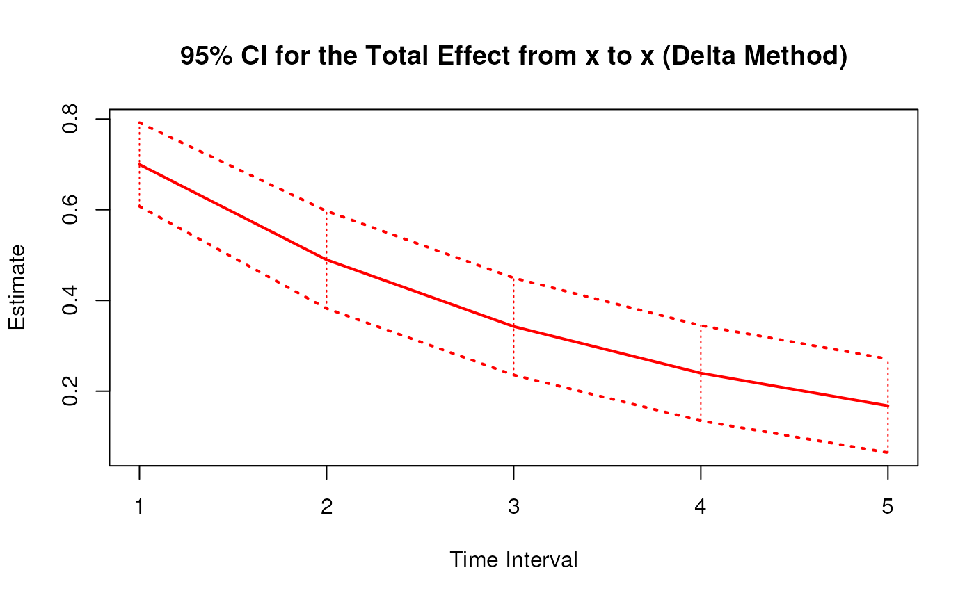
#> 1 from x to x 1 0.6998 0.0471 14.8688 0.000 0.6075 0.7920
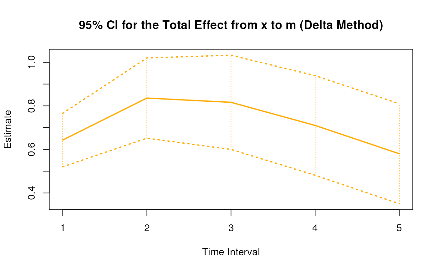
#> 2 from x to m 1 0.3888 0.0278 13.9844 0.000 0.3343 0.4433
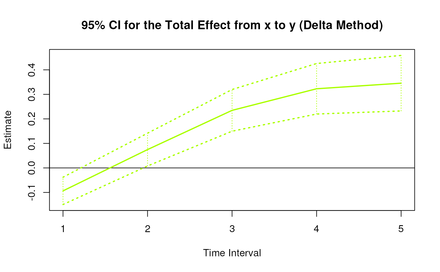
#> 3 from x to y 1 -0.1069 0.0345 -3.0977 0.002 -0.1745 -0.0393
#> 4 from m to x 1 0.0000 0.0559 0.0000 1.000 -0.1095 0.1095
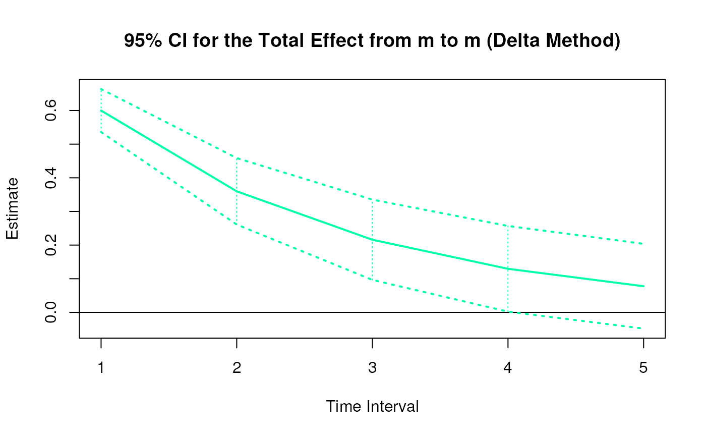
#> 5 from m to m 1 0.5999 0.0326 18.3826 0.000 0.5359 0.6639
#> 6 from m to y 1 0.5494 0.0376 14.5948 0.000 0.4756 0.6232
#> 7 from y to x 1 0.0000 0.0391 0.0000 1.000 -0.0767 0.0767
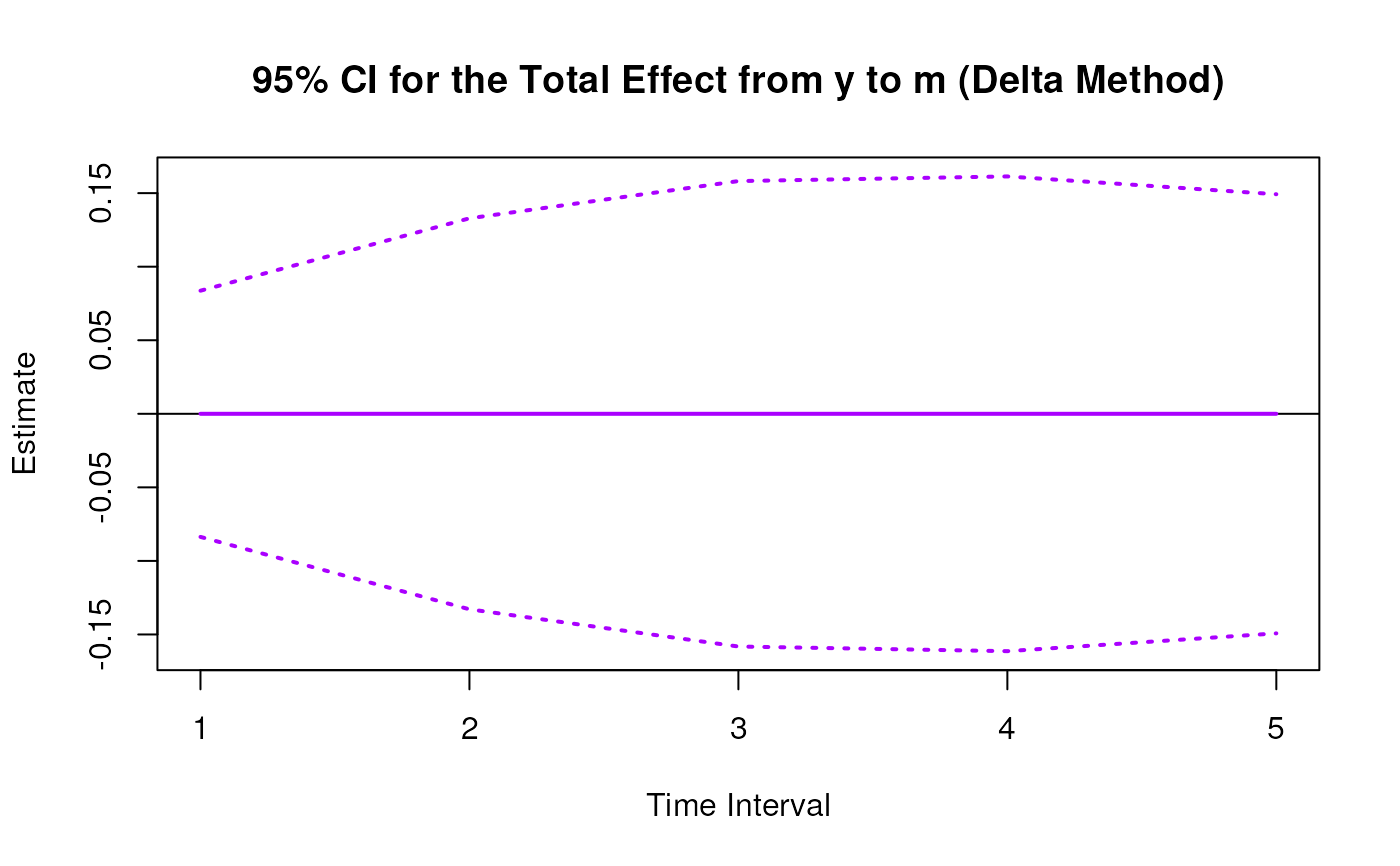
#> 8 from y to m 1 0.0000 0.0226 0.0000 1.000 -0.0443 0.0443
#> 9 from y to y 1 0.5001 0.0274 18.2776 0.000 0.4464 0.5537
# Range of time intervals ---------------------------------------------------
delta <- DeltaBetaStd(
phi = phi,
sigma = sigma,
vcov_theta = vcov_theta,
delta_t = 1:5
)
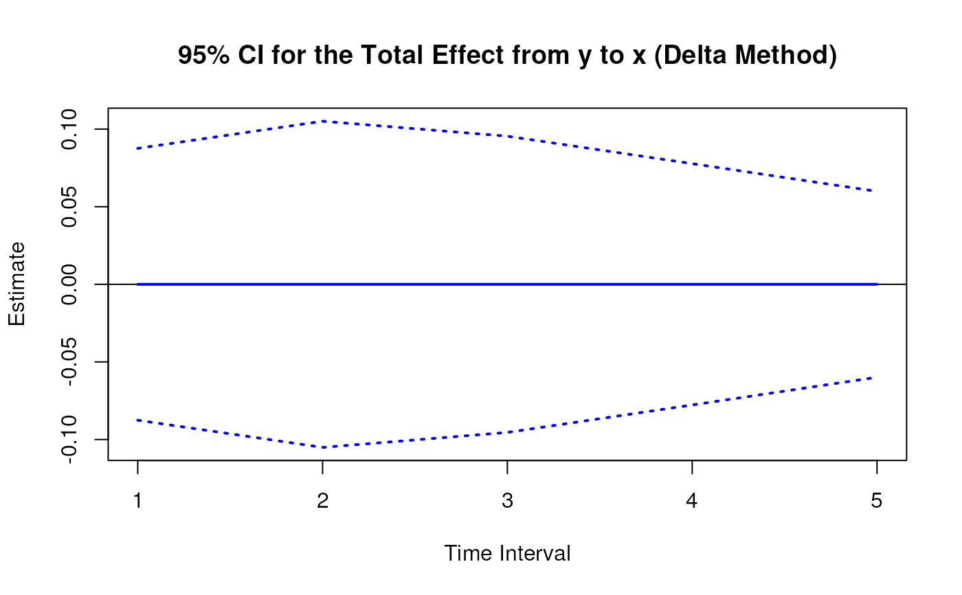
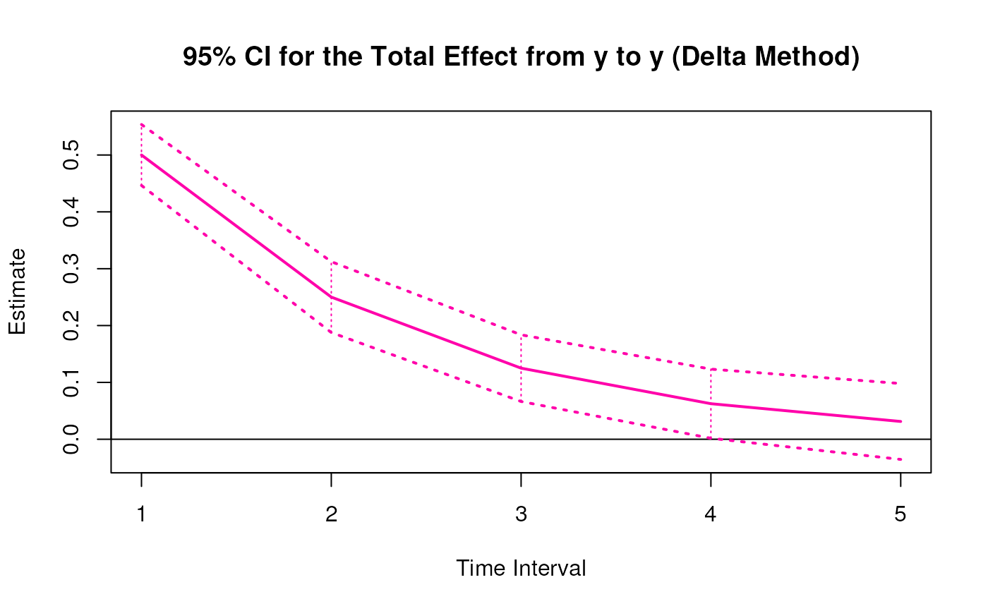
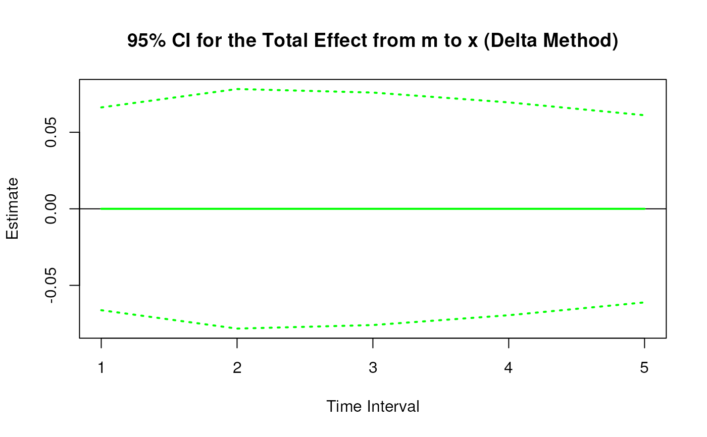
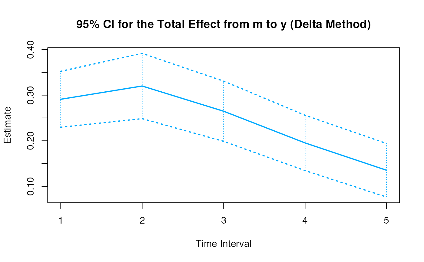
plot(delta)


 # Methods -------------------------------------------------------------------
# DeltaBetaStd has a number of methods including
# print, summary, confint, and plot
print(delta)
#> Call:
#> DeltaBetaStd(phi = phi, sigma = sigma, vcov_theta = vcov_theta,
#> delta_t = 1:5)
#>
#> Elements of the matrix of lagged coefficients
#>
#> effect interval est se z p 2.5% 97.5%
#> 1 from x to x 1 0.6998 0.0471 14.8688 0.0000 0.6075 0.7920
#> 2 from x to m 1 0.3888 0.0278 13.9844 0.0000 0.3343 0.4433
#> 3 from x to y 1 -0.1069 0.0345 -3.0977 0.0020 -0.1745 -0.0393
#> 4 from m to x 1 0.0000 0.0559 0.0000 1.0000 -0.1095 0.1095
#> 5 from m to m 1 0.5999 0.0326 18.3826 0.0000 0.5359 0.6639
#> 6 from m to y 1 0.5494 0.0376 14.5948 0.0000 0.4756 0.6232
#> 7 from y to x 1 0.0000 0.0391 0.0000 1.0000 -0.0767 0.0767
#> 8 from y to m 1 0.0000 0.0226 0.0000 1.0000 -0.0443 0.0443
#> 9 from y to y 1 0.5001 0.0274 18.2776 0.0000 0.4464 0.5537
#> 10 from x to x 2 0.4897 0.0548 8.9377 0.0000 0.3823 0.5971
#> 11 from x to m 2 0.5053 0.0381 13.2686 0.0000 0.4307 0.5800
#> 12 from x to y 2 0.0854 0.0351 2.4352 0.0149 0.0167 0.1541
#> 13 from m to x 2 0.0000 0.0660 0.0000 1.0000 -0.1294 0.1294
#> 14 from m to m 2 0.3599 0.0504 7.1405 0.0000 0.2611 0.4587
#> 15 from m to y 2 0.6044 0.0380 15.8851 0.0000 0.5298 0.6789
#> 16 from y to x 2 0.0000 0.0470 0.0000 1.0000 -0.0920 0.0920
#> 17 from y to m 2 0.0000 0.0359 0.0000 1.0000 -0.0704 0.0704
#> 18 from y to y 2 0.2501 0.0318 7.8668 0.0000 0.1878 0.3124
#> 19 from x to x 3 0.3427 0.0546 6.2779 0.0000 0.2357 0.4496
#> 20 from x to m 3 0.4936 0.0430 11.4664 0.0000 0.4092 0.5779
#> 21 from x to y 3 0.2680 0.0324 8.2632 0.0000 0.2044 0.3316
#> 22 from m to x 3 0.0000 0.0641 0.0000 1.0000 -0.1256 0.1256
#> 23 from m to m 3 0.2159 0.0609 3.5452 0.0004 0.0965 0.3352
#> 24 from m to y 3 0.4999 0.0384 13.0261 0.0000 0.4247 0.5752
#> 25 from y to x 3 0.0000 0.0426 0.0000 1.0000 -0.0836 0.0836
#> 26 from y to m 3 0.0000 0.0427 0.0000 1.0000 -0.0838 0.0838
#> 27 from y to y 3 0.1251 0.0299 4.1799 0.0000 0.0664 0.1837
#> 28 from x to x 4 0.2398 0.0536 4.4747 0.0000 0.1348 0.3448
#> 29 from x to m 4 0.4293 0.0458 9.3649 0.0000 0.3395 0.5192
#> 30 from x to y 4 0.3686 0.0346 10.6428 0.0000 0.3007 0.4364
#> 31 from m to x 4 0.0000 0.0587 0.0000 1.0000 -0.1150 0.1150
#> 32 from m to m 4 0.1295 0.0650 1.9937 0.0462 0.0022 0.2568
#> 33 from m to y 4 0.3686 0.0452 8.1496 0.0000 0.2800 0.4573
#> 34 from y to x 4 0.0000 0.0347 0.0000 1.0000 -0.0681 0.0681
#> 35 from y to m 4 0.0000 0.0436 0.0000 1.0000 -0.0855 0.0855
#> 36 from y to y 4 0.0625 0.0310 2.0161 0.0438 0.0017 0.1233
#> 37 from x to x 5 0.1678 0.0527 3.1821 0.0015 0.0644 0.2712
#> 38 from x to m 5 0.3508 0.0483 7.2628 0.0000 0.2561 0.4454
#> 39 from x to y 5 0.3946 0.0392 10.0752 0.0000 0.3178 0.4713
#> 40 from m to x 5 0.0000 0.0516 0.0000 1.0000 -0.1011 0.1011
#> 41 from m to m 5 0.0777 0.0642 1.2092 0.2266 -0.0482 0.2036
#> 42 from m to y 5 0.2555 0.0519 4.9258 0.0000 0.1538 0.3572
#> 43 from y to x 5 0.0000 0.0268 0.0000 1.0000 -0.0524 0.0524
#> 44 from y to m 5 0.0000 0.0403 0.0000 1.0000 -0.0790 0.0790
#> 45 from y to y 5 0.0313 0.0341 0.9180 0.3586 -0.0355 0.0980
summary(delta)
#> Call:
#> DeltaBetaStd(phi = phi, sigma = sigma, vcov_theta = vcov_theta,
#> delta_t = 1:5)
#>
#> Elements of the matrix of lagged coefficients
#>
#> effect interval est se z p 2.5% 97.5%
#> 1 from x to x 1 0.6998 0.0471 14.8688 0.0000 0.6075 0.7920
#> 2 from x to m 1 0.3888 0.0278 13.9844 0.0000 0.3343 0.4433
#> 3 from x to y 1 -0.1069 0.0345 -3.0977 0.0020 -0.1745 -0.0393
#> 4 from m to x 1 0.0000 0.0559 0.0000 1.0000 -0.1095 0.1095
#> 5 from m to m 1 0.5999 0.0326 18.3826 0.0000 0.5359 0.6639
#> 6 from m to y 1 0.5494 0.0376 14.5948 0.0000 0.4756 0.6232
#> 7 from y to x 1 0.0000 0.0391 0.0000 1.0000 -0.0767 0.0767
#> 8 from y to m 1 0.0000 0.0226 0.0000 1.0000 -0.0443 0.0443
#> 9 from y to y 1 0.5001 0.0274 18.2776 0.0000 0.4464 0.5537
#> 10 from x to x 2 0.4897 0.0548 8.9377 0.0000 0.3823 0.5971
#> 11 from x to m 2 0.5053 0.0381 13.2686 0.0000 0.4307 0.5800
#> 12 from x to y 2 0.0854 0.0351 2.4352 0.0149 0.0167 0.1541
#> 13 from m to x 2 0.0000 0.0660 0.0000 1.0000 -0.1294 0.1294
#> 14 from m to m 2 0.3599 0.0504 7.1405 0.0000 0.2611 0.4587
#> 15 from m to y 2 0.6044 0.0380 15.8851 0.0000 0.5298 0.6789
#> 16 from y to x 2 0.0000 0.0470 0.0000 1.0000 -0.0920 0.0920
#> 17 from y to m 2 0.0000 0.0359 0.0000 1.0000 -0.0704 0.0704
#> 18 from y to y 2 0.2501 0.0318 7.8668 0.0000 0.1878 0.3124
#> 19 from x to x 3 0.3427 0.0546 6.2779 0.0000 0.2357 0.4496
#> 20 from x to m 3 0.4936 0.0430 11.4664 0.0000 0.4092 0.5779
#> 21 from x to y 3 0.2680 0.0324 8.2632 0.0000 0.2044 0.3316
#> 22 from m to x 3 0.0000 0.0641 0.0000 1.0000 -0.1256 0.1256
#> 23 from m to m 3 0.2159 0.0609 3.5452 0.0004 0.0965 0.3352
#> 24 from m to y 3 0.4999 0.0384 13.0261 0.0000 0.4247 0.5752
#> 25 from y to x 3 0.0000 0.0426 0.0000 1.0000 -0.0836 0.0836
#> 26 from y to m 3 0.0000 0.0427 0.0000 1.0000 -0.0838 0.0838
#> 27 from y to y 3 0.1251 0.0299 4.1799 0.0000 0.0664 0.1837
#> 28 from x to x 4 0.2398 0.0536 4.4747 0.0000 0.1348 0.3448
#> 29 from x to m 4 0.4293 0.0458 9.3649 0.0000 0.3395 0.5192
#> 30 from x to y 4 0.3686 0.0346 10.6428 0.0000 0.3007 0.4364
#> 31 from m to x 4 0.0000 0.0587 0.0000 1.0000 -0.1150 0.1150
#> 32 from m to m 4 0.1295 0.0650 1.9937 0.0462 0.0022 0.2568
#> 33 from m to y 4 0.3686 0.0452 8.1496 0.0000 0.2800 0.4573
#> 34 from y to x 4 0.0000 0.0347 0.0000 1.0000 -0.0681 0.0681
#> 35 from y to m 4 0.0000 0.0436 0.0000 1.0000 -0.0855 0.0855
#> 36 from y to y 4 0.0625 0.0310 2.0161 0.0438 0.0017 0.1233
#> 37 from x to x 5 0.1678 0.0527 3.1821 0.0015 0.0644 0.2712
#> 38 from x to m 5 0.3508 0.0483 7.2628 0.0000 0.2561 0.4454
#> 39 from x to y 5 0.3946 0.0392 10.0752 0.0000 0.3178 0.4713
#> 40 from m to x 5 0.0000 0.0516 0.0000 1.0000 -0.1011 0.1011
#> 41 from m to m 5 0.0777 0.0642 1.2092 0.2266 -0.0482 0.2036
#> 42 from m to y 5 0.2555 0.0519 4.9258 0.0000 0.1538 0.3572
#> 43 from y to x 5 0.0000 0.0268 0.0000 1.0000 -0.0524 0.0524
#> 44 from y to m 5 0.0000 0.0403 0.0000 1.0000 -0.0790 0.0790
#> 45 from y to y 5 0.0313 0.0341 0.9180 0.3586 -0.0355 0.0980
confint(delta, level = 0.95)
#> effect interval 2.5 % 97.5 %
#> 1 from x to x 1 0.607530630 0.79201437
#> 2 from x to m 1 0.334329467 0.44331970
#> 3 from x to y 1 -0.174528114 -0.03925936
#> 4 from m to x 1 -0.109543659 0.10954366
#> 5 from m to m 1 0.535934031 0.66385674
#> 6 from m to y 1 0.475646549 0.62321518
#> 7 from y to x 1 -0.076701075 0.07670107
#> 8 from y to m 1 -0.044314150 0.04431415
#> 9 from y to y 1 0.446449155 0.55369804
#> 10 from x to x 2 0.382298845 0.59706425
#> 11 from x to m 2 0.430696536 0.57998911
#> 12 from x to y 2 0.016662700 0.15408968
#> 13 from m to x 2 -0.129400471 0.12940047
#> 14 from m to m 2 0.261093683 0.45865526
#> 15 from m to y 2 0.529789209 0.67892461
#> 16 from y to x 2 -0.092029485 0.09202948
#> 17 from y to m 2 -0.070374073 0.07037407
#> 18 from y to y 2 0.187769671 0.31237753
#> 19 from x to x 3 0.235686018 0.44964534
#> 20 from x to m 3 0.409189715 0.57791638
#> 21 from x to y 3 0.204433706 0.33156916
#> 22 from m to x 3 -0.125576714 0.12557671
#> 23 from m to m 3 0.096535451 0.33523862
#> 24 from m to y 3 0.424724408 0.57517374
#> 25 from y to x 3 -0.083580616 0.08358062
#> 26 from y to m 3 -0.083777370 0.08377737
#> 27 from y to y 3 0.066417023 0.18369339
#> 28 from x to x 4 0.134758701 0.34481734
#> 29 from x to m 4 0.339466162 0.51916791
#> 30 from x to y 4 0.300690166 0.43643964
#> 31 from m to x 4 -0.114968495 0.11496850
#> 32 from m to m 4 0.002192406 0.25682686
#> 33 from m to y 4 0.279972820 0.45727984
#> 34 from y to x 4 -0.068079285 0.06807929
#> 35 from y to m 4 -0.085451786 0.08545179
#> 36 from y to y 4 0.001740919 0.12333269
#> 37 from x to x 5 0.064444048 0.27115007
#> 38 from x to m 5 0.256117592 0.44544398
#> 39 from x to y 5 0.317802836 0.47131270
#> 40 from m to x 5 -0.101102763 0.10110276
#> 41 from m to m 5 -0.048232879 0.20361734
#> 42 from m to y 5 0.153836016 0.35715776
#> 43 from y to x 5 -0.052436652 0.05243665
#> 44 from y to m 5 -0.079042272 0.07904227
#> 45 from y to y 5 -0.035495583 0.09804159
plot(delta)
# Methods -------------------------------------------------------------------
# DeltaBetaStd has a number of methods including
# print, summary, confint, and plot
print(delta)
#> Call:
#> DeltaBetaStd(phi = phi, sigma = sigma, vcov_theta = vcov_theta,
#> delta_t = 1:5)
#>
#> Elements of the matrix of lagged coefficients
#>
#> effect interval est se z p 2.5% 97.5%
#> 1 from x to x 1 0.6998 0.0471 14.8688 0.0000 0.6075 0.7920
#> 2 from x to m 1 0.3888 0.0278 13.9844 0.0000 0.3343 0.4433
#> 3 from x to y 1 -0.1069 0.0345 -3.0977 0.0020 -0.1745 -0.0393
#> 4 from m to x 1 0.0000 0.0559 0.0000 1.0000 -0.1095 0.1095
#> 5 from m to m 1 0.5999 0.0326 18.3826 0.0000 0.5359 0.6639
#> 6 from m to y 1 0.5494 0.0376 14.5948 0.0000 0.4756 0.6232
#> 7 from y to x 1 0.0000 0.0391 0.0000 1.0000 -0.0767 0.0767
#> 8 from y to m 1 0.0000 0.0226 0.0000 1.0000 -0.0443 0.0443
#> 9 from y to y 1 0.5001 0.0274 18.2776 0.0000 0.4464 0.5537
#> 10 from x to x 2 0.4897 0.0548 8.9377 0.0000 0.3823 0.5971
#> 11 from x to m 2 0.5053 0.0381 13.2686 0.0000 0.4307 0.5800
#> 12 from x to y 2 0.0854 0.0351 2.4352 0.0149 0.0167 0.1541
#> 13 from m to x 2 0.0000 0.0660 0.0000 1.0000 -0.1294 0.1294
#> 14 from m to m 2 0.3599 0.0504 7.1405 0.0000 0.2611 0.4587
#> 15 from m to y 2 0.6044 0.0380 15.8851 0.0000 0.5298 0.6789
#> 16 from y to x 2 0.0000 0.0470 0.0000 1.0000 -0.0920 0.0920
#> 17 from y to m 2 0.0000 0.0359 0.0000 1.0000 -0.0704 0.0704
#> 18 from y to y 2 0.2501 0.0318 7.8668 0.0000 0.1878 0.3124
#> 19 from x to x 3 0.3427 0.0546 6.2779 0.0000 0.2357 0.4496
#> 20 from x to m 3 0.4936 0.0430 11.4664 0.0000 0.4092 0.5779
#> 21 from x to y 3 0.2680 0.0324 8.2632 0.0000 0.2044 0.3316
#> 22 from m to x 3 0.0000 0.0641 0.0000 1.0000 -0.1256 0.1256
#> 23 from m to m 3 0.2159 0.0609 3.5452 0.0004 0.0965 0.3352
#> 24 from m to y 3 0.4999 0.0384 13.0261 0.0000 0.4247 0.5752
#> 25 from y to x 3 0.0000 0.0426 0.0000 1.0000 -0.0836 0.0836
#> 26 from y to m 3 0.0000 0.0427 0.0000 1.0000 -0.0838 0.0838
#> 27 from y to y 3 0.1251 0.0299 4.1799 0.0000 0.0664 0.1837
#> 28 from x to x 4 0.2398 0.0536 4.4747 0.0000 0.1348 0.3448
#> 29 from x to m 4 0.4293 0.0458 9.3649 0.0000 0.3395 0.5192
#> 30 from x to y 4 0.3686 0.0346 10.6428 0.0000 0.3007 0.4364
#> 31 from m to x 4 0.0000 0.0587 0.0000 1.0000 -0.1150 0.1150
#> 32 from m to m 4 0.1295 0.0650 1.9937 0.0462 0.0022 0.2568
#> 33 from m to y 4 0.3686 0.0452 8.1496 0.0000 0.2800 0.4573
#> 34 from y to x 4 0.0000 0.0347 0.0000 1.0000 -0.0681 0.0681
#> 35 from y to m 4 0.0000 0.0436 0.0000 1.0000 -0.0855 0.0855
#> 36 from y to y 4 0.0625 0.0310 2.0161 0.0438 0.0017 0.1233
#> 37 from x to x 5 0.1678 0.0527 3.1821 0.0015 0.0644 0.2712
#> 38 from x to m 5 0.3508 0.0483 7.2628 0.0000 0.2561 0.4454
#> 39 from x to y 5 0.3946 0.0392 10.0752 0.0000 0.3178 0.4713
#> 40 from m to x 5 0.0000 0.0516 0.0000 1.0000 -0.1011 0.1011
#> 41 from m to m 5 0.0777 0.0642 1.2092 0.2266 -0.0482 0.2036
#> 42 from m to y 5 0.2555 0.0519 4.9258 0.0000 0.1538 0.3572
#> 43 from y to x 5 0.0000 0.0268 0.0000 1.0000 -0.0524 0.0524
#> 44 from y to m 5 0.0000 0.0403 0.0000 1.0000 -0.0790 0.0790
#> 45 from y to y 5 0.0313 0.0341 0.9180 0.3586 -0.0355 0.0980
summary(delta)
#> Call:
#> DeltaBetaStd(phi = phi, sigma = sigma, vcov_theta = vcov_theta,
#> delta_t = 1:5)
#>
#> Elements of the matrix of lagged coefficients
#>
#> effect interval est se z p 2.5% 97.5%
#> 1 from x to x 1 0.6998 0.0471 14.8688 0.0000 0.6075 0.7920
#> 2 from x to m 1 0.3888 0.0278 13.9844 0.0000 0.3343 0.4433
#> 3 from x to y 1 -0.1069 0.0345 -3.0977 0.0020 -0.1745 -0.0393
#> 4 from m to x 1 0.0000 0.0559 0.0000 1.0000 -0.1095 0.1095
#> 5 from m to m 1 0.5999 0.0326 18.3826 0.0000 0.5359 0.6639
#> 6 from m to y 1 0.5494 0.0376 14.5948 0.0000 0.4756 0.6232
#> 7 from y to x 1 0.0000 0.0391 0.0000 1.0000 -0.0767 0.0767
#> 8 from y to m 1 0.0000 0.0226 0.0000 1.0000 -0.0443 0.0443
#> 9 from y to y 1 0.5001 0.0274 18.2776 0.0000 0.4464 0.5537
#> 10 from x to x 2 0.4897 0.0548 8.9377 0.0000 0.3823 0.5971
#> 11 from x to m 2 0.5053 0.0381 13.2686 0.0000 0.4307 0.5800
#> 12 from x to y 2 0.0854 0.0351 2.4352 0.0149 0.0167 0.1541
#> 13 from m to x 2 0.0000 0.0660 0.0000 1.0000 -0.1294 0.1294
#> 14 from m to m 2 0.3599 0.0504 7.1405 0.0000 0.2611 0.4587
#> 15 from m to y 2 0.6044 0.0380 15.8851 0.0000 0.5298 0.6789
#> 16 from y to x 2 0.0000 0.0470 0.0000 1.0000 -0.0920 0.0920
#> 17 from y to m 2 0.0000 0.0359 0.0000 1.0000 -0.0704 0.0704
#> 18 from y to y 2 0.2501 0.0318 7.8668 0.0000 0.1878 0.3124
#> 19 from x to x 3 0.3427 0.0546 6.2779 0.0000 0.2357 0.4496
#> 20 from x to m 3 0.4936 0.0430 11.4664 0.0000 0.4092 0.5779
#> 21 from x to y 3 0.2680 0.0324 8.2632 0.0000 0.2044 0.3316
#> 22 from m to x 3 0.0000 0.0641 0.0000 1.0000 -0.1256 0.1256
#> 23 from m to m 3 0.2159 0.0609 3.5452 0.0004 0.0965 0.3352
#> 24 from m to y 3 0.4999 0.0384 13.0261 0.0000 0.4247 0.5752
#> 25 from y to x 3 0.0000 0.0426 0.0000 1.0000 -0.0836 0.0836
#> 26 from y to m 3 0.0000 0.0427 0.0000 1.0000 -0.0838 0.0838
#> 27 from y to y 3 0.1251 0.0299 4.1799 0.0000 0.0664 0.1837
#> 28 from x to x 4 0.2398 0.0536 4.4747 0.0000 0.1348 0.3448
#> 29 from x to m 4 0.4293 0.0458 9.3649 0.0000 0.3395 0.5192
#> 30 from x to y 4 0.3686 0.0346 10.6428 0.0000 0.3007 0.4364
#> 31 from m to x 4 0.0000 0.0587 0.0000 1.0000 -0.1150 0.1150
#> 32 from m to m 4 0.1295 0.0650 1.9937 0.0462 0.0022 0.2568
#> 33 from m to y 4 0.3686 0.0452 8.1496 0.0000 0.2800 0.4573
#> 34 from y to x 4 0.0000 0.0347 0.0000 1.0000 -0.0681 0.0681
#> 35 from y to m 4 0.0000 0.0436 0.0000 1.0000 -0.0855 0.0855
#> 36 from y to y 4 0.0625 0.0310 2.0161 0.0438 0.0017 0.1233
#> 37 from x to x 5 0.1678 0.0527 3.1821 0.0015 0.0644 0.2712
#> 38 from x to m 5 0.3508 0.0483 7.2628 0.0000 0.2561 0.4454
#> 39 from x to y 5 0.3946 0.0392 10.0752 0.0000 0.3178 0.4713
#> 40 from m to x 5 0.0000 0.0516 0.0000 1.0000 -0.1011 0.1011
#> 41 from m to m 5 0.0777 0.0642 1.2092 0.2266 -0.0482 0.2036
#> 42 from m to y 5 0.2555 0.0519 4.9258 0.0000 0.1538 0.3572
#> 43 from y to x 5 0.0000 0.0268 0.0000 1.0000 -0.0524 0.0524
#> 44 from y to m 5 0.0000 0.0403 0.0000 1.0000 -0.0790 0.0790
#> 45 from y to y 5 0.0313 0.0341 0.9180 0.3586 -0.0355 0.0980
confint(delta, level = 0.95)
#> effect interval 2.5 % 97.5 %
#> 1 from x to x 1 0.607530630 0.79201437
#> 2 from x to m 1 0.334329467 0.44331970
#> 3 from x to y 1 -0.174528114 -0.03925936
#> 4 from m to x 1 -0.109543659 0.10954366
#> 5 from m to m 1 0.535934031 0.66385674
#> 6 from m to y 1 0.475646549 0.62321518
#> 7 from y to x 1 -0.076701075 0.07670107
#> 8 from y to m 1 -0.044314150 0.04431415
#> 9 from y to y 1 0.446449155 0.55369804
#> 10 from x to x 2 0.382298845 0.59706425
#> 11 from x to m 2 0.430696536 0.57998911
#> 12 from x to y 2 0.016662700 0.15408968
#> 13 from m to x 2 -0.129400471 0.12940047
#> 14 from m to m 2 0.261093683 0.45865526
#> 15 from m to y 2 0.529789209 0.67892461
#> 16 from y to x 2 -0.092029485 0.09202948
#> 17 from y to m 2 -0.070374073 0.07037407
#> 18 from y to y 2 0.187769671 0.31237753
#> 19 from x to x 3 0.235686018 0.44964534
#> 20 from x to m 3 0.409189715 0.57791638
#> 21 from x to y 3 0.204433706 0.33156916
#> 22 from m to x 3 -0.125576714 0.12557671
#> 23 from m to m 3 0.096535451 0.33523862
#> 24 from m to y 3 0.424724408 0.57517374
#> 25 from y to x 3 -0.083580616 0.08358062
#> 26 from y to m 3 -0.083777370 0.08377737
#> 27 from y to y 3 0.066417023 0.18369339
#> 28 from x to x 4 0.134758701 0.34481734
#> 29 from x to m 4 0.339466162 0.51916791
#> 30 from x to y 4 0.300690166 0.43643964
#> 31 from m to x 4 -0.114968495 0.11496850
#> 32 from m to m 4 0.002192406 0.25682686
#> 33 from m to y 4 0.279972820 0.45727984
#> 34 from y to x 4 -0.068079285 0.06807929
#> 35 from y to m 4 -0.085451786 0.08545179
#> 36 from y to y 4 0.001740919 0.12333269
#> 37 from x to x 5 0.064444048 0.27115007
#> 38 from x to m 5 0.256117592 0.44544398
#> 39 from x to y 5 0.317802836 0.47131270
#> 40 from m to x 5 -0.101102763 0.10110276
#> 41 from m to m 5 -0.048232879 0.20361734
#> 42 from m to y 5 0.153836016 0.35715776
#> 43 from y to x 5 -0.052436652 0.05243665
#> 44 from y to m 5 -0.079042272 0.07904227
#> 45 from y to y 5 -0.035495583 0.09804159
plot(delta)