Posterior Distribution of the Indirect Effect Centrality Over a Specific Time Interval or a Range of Time Intervals
Source:R/cTMed-posterior-indirect-central.R
PosteriorIndirectCentral.RdThis function generates a posterior distribution of the indirect effect centrality over a specific time interval \(\Delta t\) or a range of time intervals using the posterior distribution of the first-order stochastic differential equation model drift matrix \(\boldsymbol{\Phi}\).
Arguments
- phi
List of numeric matrices. Each element of the list is a sample from the posterior distribution of the drift matrix (\(\boldsymbol{\Phi}\)). Each matrix should have row and column names pertaining to the variables in the system.
- delta_t
Numeric. Time interval (\(\Delta t\)).
- ncores
Positive integer. Number of cores to use. If
ncores = NULL, use a single core. Consider using multiple cores when number of replicationsRis a large value.- tol
Numeric. Smallest possible time interval to allow.
Value
Returns an object
of class ctmedmc which is a list with the following elements:
- call
Function call.
- args
Function arguments.
- fun
Function used ("PosteriorIndirectCentral").
- output
A list of length
length(delta_t).
Each element in the output list has the following elements:
- est
Mean of the posterior distribution of the indirect effect centrality.
- thetahatstar
Posterior distribution of the indirect effect centrality measure.
Details
See IndirectCentral() for more details.
References
Bollen, K. A. (1987). Total, direct, and indirect effects in structural equation models. Sociological Methodology, 17, 37. doi:10.2307/271028
Deboeck, P. R., & Preacher, K. J. (2015). No need to be discrete: A method for continuous time mediation analysis. Structural Equation Modeling: A Multidisciplinary Journal, 23 (1), 61-75. doi:10.1080/10705511.2014.973960
Pesigan, I. J. A., Russell, M. A., & Chow, S.-M. (2025). Inferences and effect sizes for direct, indirect, and total effects in continuous-time mediation models. Psychological Methods. doi:10.1037/met0000779
Ryan, O., & Hamaker, E. L. (2021). Time to intervene: A continuous-time approach to network analysis and centrality. Psychometrika, 87 (1), 214-252. doi:10.1007/s11336-021-09767-0
See also
Other Continuous-Time Mediation Functions:
BootBeta(),
BootBetaStd(),
BootDirectCentral(),
BootDirectCentralStd(),
BootIndirectCentral(),
BootIndirectCentralStd(),
BootMed(),
BootMedStd(),
BootTotalCentral(),
BootTotalCentralStd(),
DeltaBeta(),
DeltaBetaStd(),
DeltaDirectCentral(),
DeltaDirectCentralStd(),
DeltaIndirectCentral(),
DeltaMed(),
DeltaMedStd(),
DeltaTotalCentral(),
DeltaTotalCentralStd(),
Direct(),
DirectCentral(),
DirectCentralStd(),
DirectStd(),
Indirect(),
IndirectCentral(),
IndirectCentralStd(),
IndirectStd(),
MCBeta(),
MCBetaStd(),
MCDirectCentral(),
MCDirectCentralStd(),
MCIndirectCentral(),
MCIndirectCentralStd(),
MCMed(),
MCMedStd(),
MCPhi(),
MCPhiSigma(),
MCTotalCentral(),
MCTotalCentralStd(),
Med(),
MedStd(),
PosteriorBeta(),
PosteriorBetaStd(),
PosteriorDirectCentral(),
PosteriorDirectCentralStd(),
PosteriorIndirectCentralStd(),
PosteriorMed(),
PosteriorMedStd(),
PosteriorTotalCentral(),
PosteriorTotalCentralStd(),
Total(),
TotalCentral(),
TotalCentralStd(),
TotalStd(),
Trajectory()
Examples
phi <- matrix(
data = c(
-0.357, 0.771, -0.450,
0.0, -0.511, 0.729,
0, 0, -0.693
),
nrow = 3
)
colnames(phi) <- rownames(phi) <- c("x", "m", "y")
vcov_phi_vec <- matrix(
data = c(
0.00843, 0.00040, -0.00151,
-0.00600, -0.00033, 0.00110,
0.00324, 0.00020, -0.00061,
0.00040, 0.00374, 0.00016,
-0.00022, -0.00273, -0.00016,
0.00009, 0.00150, 0.00012,
-0.00151, 0.00016, 0.00389,
0.00103, -0.00007, -0.00283,
-0.00050, 0.00000, 0.00156,
-0.00600, -0.00022, 0.00103,
0.00644, 0.00031, -0.00119,
-0.00374, -0.00021, 0.00070,
-0.00033, -0.00273, -0.00007,
0.00031, 0.00287, 0.00013,
-0.00014, -0.00170, -0.00012,
0.00110, -0.00016, -0.00283,
-0.00119, 0.00013, 0.00297,
0.00063, -0.00004, -0.00177,
0.00324, 0.00009, -0.00050,
-0.00374, -0.00014, 0.00063,
0.00495, 0.00024, -0.00093,
0.00020, 0.00150, 0.00000,
-0.00021, -0.00170, -0.00004,
0.00024, 0.00214, 0.00012,
-0.00061, 0.00012, 0.00156,
0.00070, -0.00012, -0.00177,
-0.00093, 0.00012, 0.00223
),
nrow = 9
)
phi <- MCPhi(
phi = phi,
vcov_phi_vec = vcov_phi_vec,
R = 1000L
)$output
# Specific time interval ----------------------------------------------------
PosteriorIndirectCentral(
phi = phi,
delta_t = 1
)
#> Call:
#> PosteriorIndirectCentral(phi = phi, delta_t = 1)
#>
#> Indirect Effect Centrality
#> variable interval est se R 2.5% 97.5%
#> 1 x 1 0.0004 0.0197 1000 -0.0381 0.0393
#> 2 m 1 0.1663 0.0174 1000 0.1331 0.2023
#> 3 y 1 0.0007 0.0141 1000 -0.0252 0.0291
# Range of time intervals ---------------------------------------------------
posterior <- PosteriorIndirectCentral(
phi = phi,
delta_t = 1:5
)
# Methods -------------------------------------------------------------------
# PosteriorIndirectCentral has a number of methods including
# print, summary, confint, and plot
print(posterior)
#> Call:
#> PosteriorIndirectCentral(phi = phi, delta_t = 1:5)
#>
#> Indirect Effect Centrality
#> variable interval est se R 2.5% 97.5%
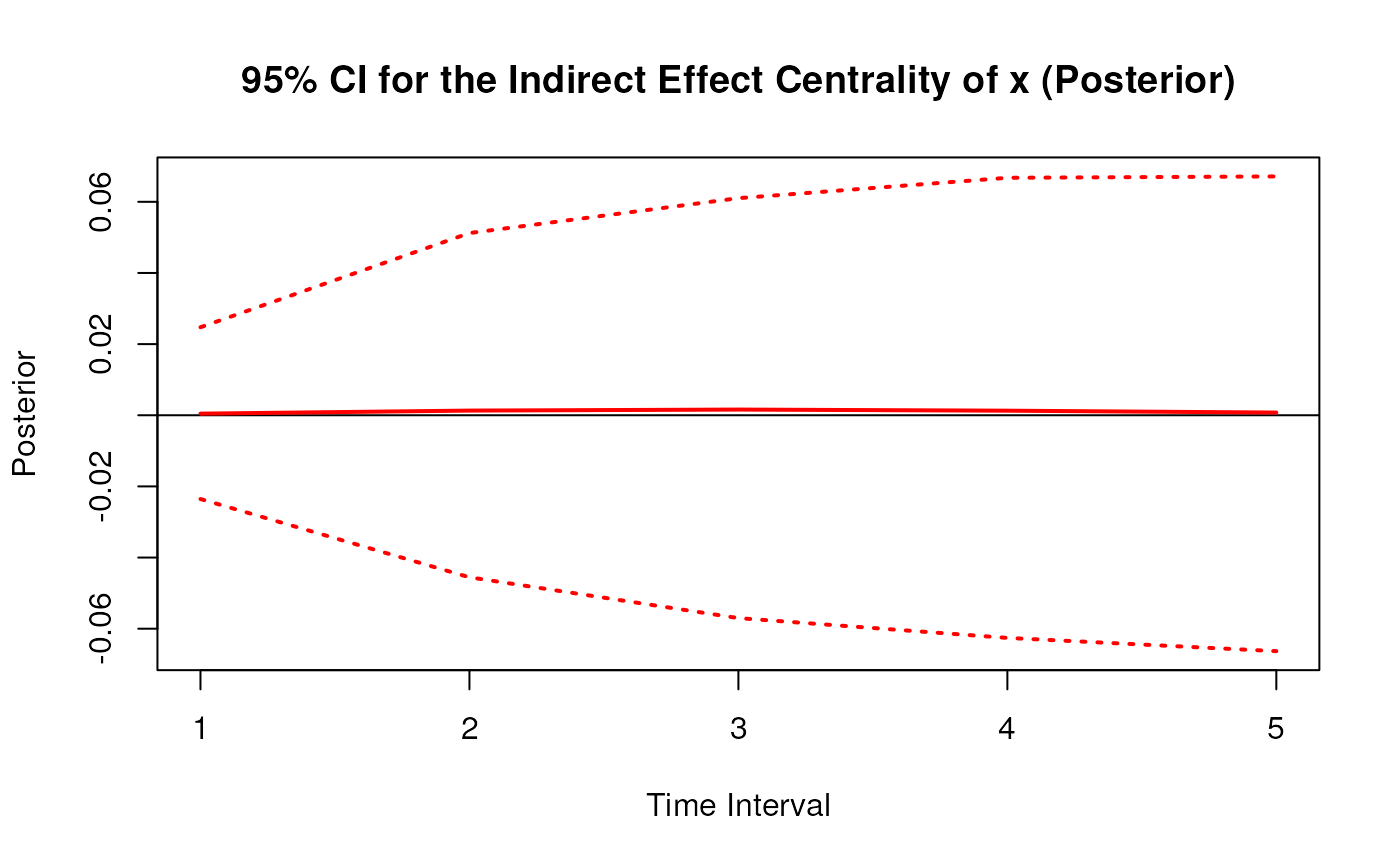
#> 1 x 1 0.0004 0.0197 1000 -0.0381 0.0393
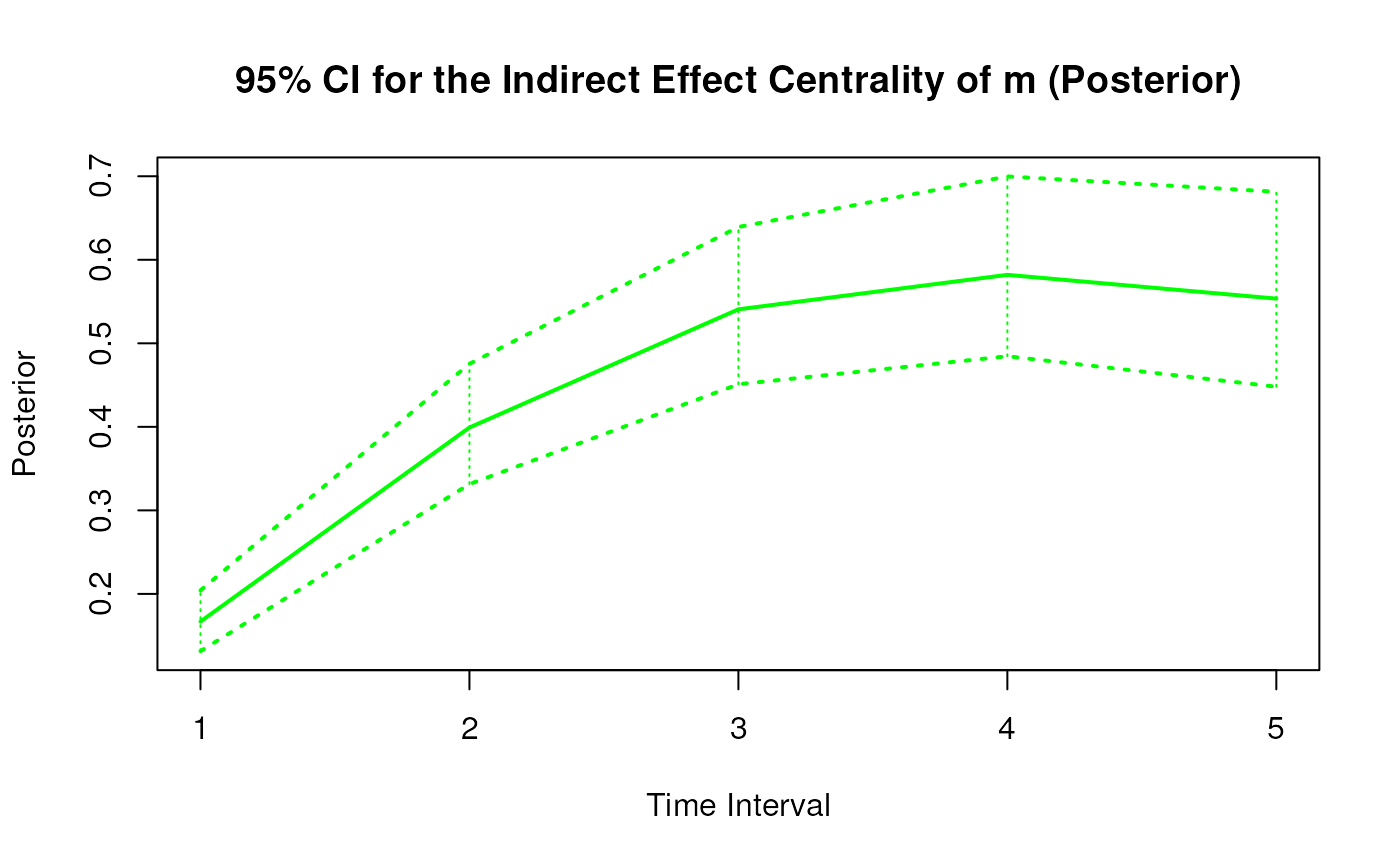
#> 2 m 1 0.1663 0.0174 1000 0.1331 0.2023
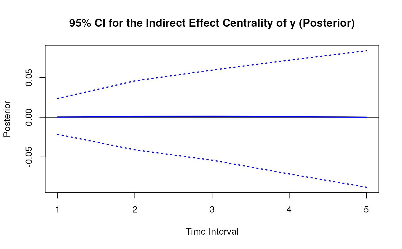
#> 3 y 1 0.0007 0.0141 1000 -0.0252 0.0291
#> 4 x 2 0.0009 0.0387 1000 -0.0740 0.0749
#> 5 m 2 0.3989 0.0456 1000 0.3144 0.4928
#> 6 y 2 0.0016 0.0326 1000 -0.0593 0.0686
#> 7 x 3 0.0008 0.0472 1000 -0.0928 0.0881
#> 8 m 3 0.5420 0.0704 1000 0.4173 0.6907
#> 9 y 3 0.0017 0.0491 1000 -0.0924 0.0955
#> 10 x 4 0.0007 0.0519 1000 -0.1025 0.0993
#> 11 m 4 0.5859 0.0868 1000 0.4402 0.7669
#> 12 y 4 0.0009 0.0655 1000 -0.1289 0.1203
#> 13 x 5 0.0007 0.0558 1000 -0.1090 0.1081
#> 14 m 5 0.5603 0.0939 1000 0.4052 0.7656
#> 15 y 5 -0.0002 0.0809 1000 -0.1654 0.1441
summary(posterior)
#> Call:
#> PosteriorIndirectCentral(phi = phi, delta_t = 1:5)
#>
#> Indirect Effect Centrality
#> variable interval est se R 2.5% 97.5%
#> 1 x 1 0.0004 0.0197 1000 -0.0381 0.0393
#> 2 m 1 0.1663 0.0174 1000 0.1331 0.2023
#> 3 y 1 0.0007 0.0141 1000 -0.0252 0.0291
#> 4 x 2 0.0009 0.0387 1000 -0.0740 0.0749
#> 5 m 2 0.3989 0.0456 1000 0.3144 0.4928
#> 6 y 2 0.0016 0.0326 1000 -0.0593 0.0686
#> 7 x 3 0.0008 0.0472 1000 -0.0928 0.0881
#> 8 m 3 0.5420 0.0704 1000 0.4173 0.6907
#> 9 y 3 0.0017 0.0491 1000 -0.0924 0.0955
#> 10 x 4 0.0007 0.0519 1000 -0.1025 0.0993
#> 11 m 4 0.5859 0.0868 1000 0.4402 0.7669
#> 12 y 4 0.0009 0.0655 1000 -0.1289 0.1203
#> 13 x 5 0.0007 0.0558 1000 -0.1090 0.1081
#> 14 m 5 0.5603 0.0939 1000 0.4052 0.7656
#> 15 y 5 -0.0002 0.0809 1000 -0.1654 0.1441
confint(posterior, level = 0.95)
#> variable interval 2.5 % 97.5 %
#> 1 x 1 -0.03811420 0.03929921
#> 2 m 1 0.13314348 0.20227304
#> 3 y 1 -0.02518484 0.02908187
#> 4 x 2 -0.07399302 0.07488532
#> 5 m 2 0.31441622 0.49283213
#> 6 y 2 -0.05928478 0.06862402
#> 7 x 3 -0.09284279 0.08809300
#> 8 m 3 0.41726255 0.69070716
#> 9 y 3 -0.09235517 0.09548283
#> 10 x 4 -0.10249765 0.09932252
#> 11 m 4 0.44017002 0.76688151
#> 12 y 4 -0.12893029 0.12029253
#> 13 x 5 -0.10899640 0.10814922
#> 14 m 5 0.40515295 0.76563430
#> 15 y 5 -0.16544337 0.14409441
plot(posterior)