Direct Effect Centrality
Value
Returns an object
of class ctmedmed which is a list with the following elements:
- call
Function call.
- args
Function arguments.
- fun
Function used ("DirectCentral").
- output
A matrix of direct effect centrality.
Details
Direct effect centrality is the sum of all possible direct effects between different pairs of variables in which a specific variable serves as the only mediator.
References
Bollen, K. A. (1987). Total, direct, and indirect effects in structural equation models. Sociological Methodology, 17, 37. doi:10.2307/271028
Deboeck, P. R., & Preacher, K. J. (2015). No need to be discrete: A method for continuous time mediation analysis. Structural Equation Modeling: A Multidisciplinary Journal, 23 (1), 61-75. doi:10.1080/10705511.2014.973960
Pesigan, I. J. A., Russell, M. A., & Chow, S.-M. (2025). Inferences and effect sizes for direct, indirect, and total effects in continuous-time mediation models. Psychological Methods. doi:10.1037/met0000779
Ryan, O., & Hamaker, E. L. (2021). Time to intervene: A continuous-time approach to network analysis and centrality. Psychometrika, 87 (1), 214-252. doi:10.1007/s11336-021-09767-0
See also
Other Continuous-Time Mediation Functions:
BootBeta(),
BootBetaStd(),
BootDirectCentral(),
BootDirectCentralStd(),
BootIndirectCentral(),
BootIndirectCentralStd(),
BootMed(),
BootMedStd(),
BootTotalCentral(),
BootTotalCentralStd(),
DeltaBeta(),
DeltaBetaStd(),
DeltaDirectCentral(),
DeltaDirectCentralStd(),
DeltaIndirectCentral(),
DeltaMed(),
DeltaMedStd(),
DeltaTotalCentral(),
DeltaTotalCentralStd(),
Direct(),
DirectCentralStd(),
DirectStd(),
Indirect(),
IndirectCentral(),
IndirectCentralStd(),
IndirectStd(),
MCBeta(),
MCBetaStd(),
MCDirectCentral(),
MCDirectCentralStd(),
MCIndirectCentral(),
MCIndirectCentralStd(),
MCMed(),
MCMedStd(),
MCPhi(),
MCPhiSigma(),
MCTotalCentral(),
MCTotalCentralStd(),
Med(),
MedStd(),
PosteriorBeta(),
PosteriorBetaStd(),
PosteriorDirectCentral(),
PosteriorDirectCentralStd(),
PosteriorIndirectCentral(),
PosteriorIndirectCentralStd(),
PosteriorMed(),
PosteriorMedStd(),
PosteriorTotalCentral(),
PosteriorTotalCentralStd(),
Total(),
TotalCentral(),
TotalCentralStd(),
TotalStd(),
Trajectory()
Examples
phi <- matrix(
data = c(
-0.357, 0.771, -0.450,
0.0, -0.511, 0.729,
0, 0, -0.693
),
nrow = 3
)
colnames(phi) <- rownames(phi) <- c("x", "m", "y")
# Specific time interval ----------------------------------------------------
DirectCentral(
phi = phi,
delta_t = 1
)
#> Call:
#> DirectCentral(phi = phi, delta_t = 1)
#>
#> Direct Effect Centrality
#> interval x m y
#> [1,] 1 0.3998 -0.2675 0.5
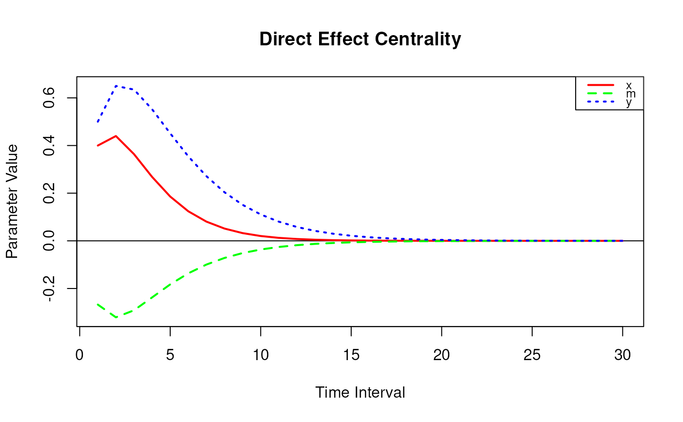
# Range of time intervals ---------------------------------------------------
direct_central <- DirectCentral(
phi = phi,
delta_t = 1:30
)
plot(direct_central)
 # Methods -------------------------------------------------------------------
# DirectCentral has a number of methods including
# print, summary, and plot
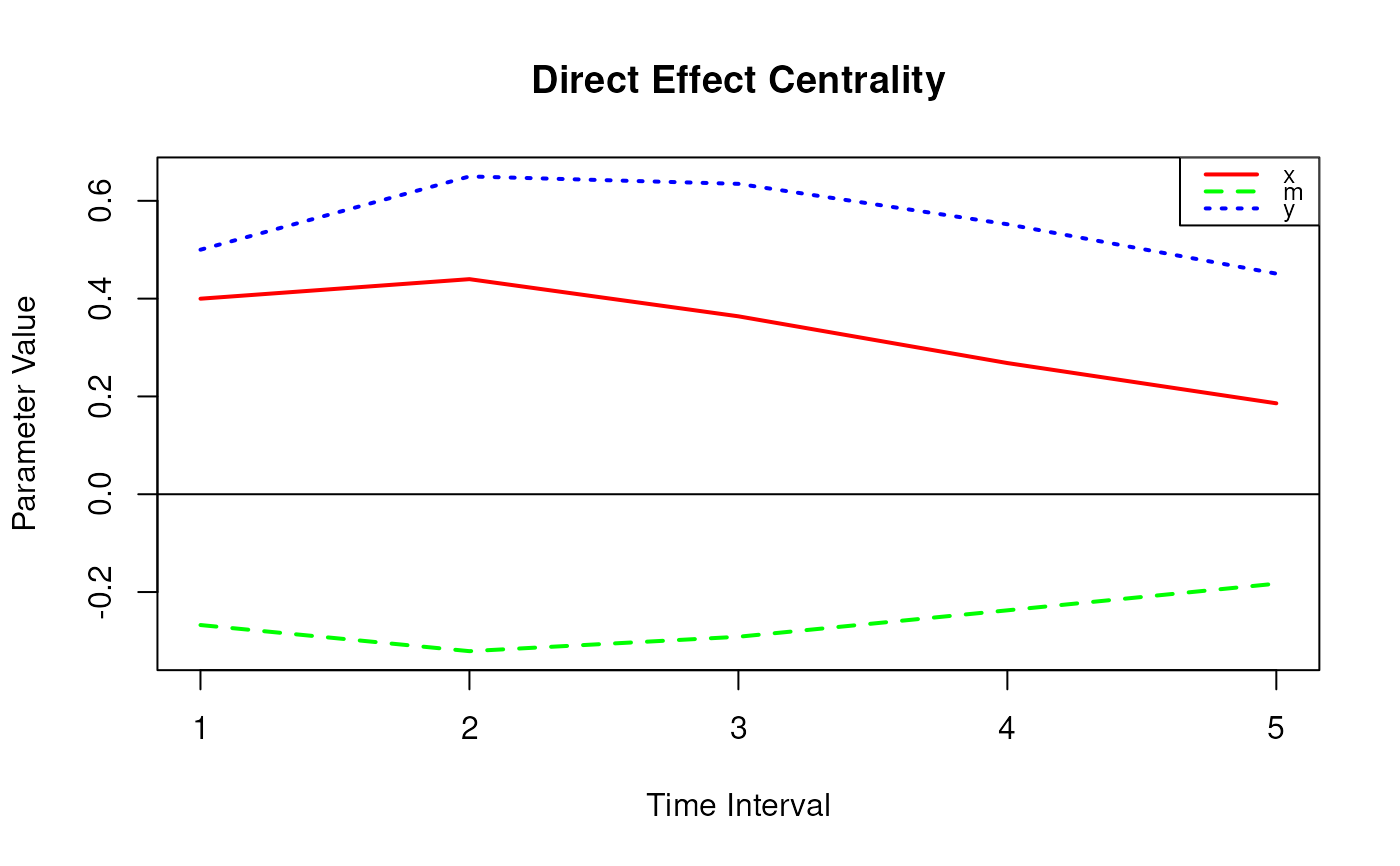
direct_central <- DirectCentral(
phi = phi,
delta_t = 1:5
)
print(direct_central)
#> Call:
#> DirectCentral(phi = phi, delta_t = 1:5)
#>
#> Direct Effect Centrality
#> interval x m y
#> [1,] 1 0.3998 -0.2675 0.5000
#> [2,] 2 0.4398 -0.3209 0.6499
#> [3,] 3 0.3638 -0.2914 0.6347
#> [4,] 4 0.2683 -0.2374 0.5521
#> [5,] 5 0.1859 -0.1828 0.4511
summary(direct_central)
#> Call:
#> DirectCentral(phi = phi, delta_t = 1:5)
#>
#> Direct Effect Centrality
#> interval x m y
#> [1,] 1 0.3998 -0.2675 0.5000
#> [2,] 2 0.4398 -0.3209 0.6499
#> [3,] 3 0.3638 -0.2914 0.6347
#> [4,] 4 0.2683 -0.2374 0.5521
#> [5,] 5 0.1859 -0.1828 0.4511
plot(direct_central)
# Methods -------------------------------------------------------------------
# DirectCentral has a number of methods including
# print, summary, and plot
direct_central <- DirectCentral(
phi = phi,
delta_t = 1:5
)
print(direct_central)
#> Call:
#> DirectCentral(phi = phi, delta_t = 1:5)
#>
#> Direct Effect Centrality
#> interval x m y
#> [1,] 1 0.3998 -0.2675 0.5000
#> [2,] 2 0.4398 -0.3209 0.6499
#> [3,] 3 0.3638 -0.2914 0.6347
#> [4,] 4 0.2683 -0.2374 0.5521
#> [5,] 5 0.1859 -0.1828 0.4511
summary(direct_central)
#> Call:
#> DirectCentral(phi = phi, delta_t = 1:5)
#>
#> Direct Effect Centrality
#> interval x m y
#> [1,] 1 0.3998 -0.2675 0.5000
#> [2,] 2 0.4398 -0.3209 0.6499
#> [3,] 3 0.3638 -0.2914 0.6347
#> [4,] 4 0.2683 -0.2374 0.5521
#> [5,] 5 0.1859 -0.1828 0.4511
plot(direct_central)