Posterior Distribution of the Direct Effect Centrality Over a Specific Time Interval or a Range of Time Intervals
Source:R/cTMed-posterior-direct-central.R
PosteriorDirectCentral.RdThis function generates a posterior distribution of the direct effect centrality over a specific time interval \(\Delta t\) or a range of time intervals using the posterior distribution of the first-order stochastic differential equation model drift matrix \(\boldsymbol{\Phi}\).
Arguments
- phi
List of numeric matrices. Each element of the list is a sample from the posterior distribution of the drift matrix (\(\boldsymbol{\Phi}\)). Each matrix should have row and column names pertaining to the variables in the system.
- delta_t
Numeric. Time interval (\(\Delta t\)).
- ncores
Positive integer. Number of cores to use. If
ncores = NULL, use a single core. Consider using multiple cores when number of replicationsRis a large value.- tol
Numeric. Smallest possible time interval to allow.
Value
Returns an object
of class ctmedmc which is a list with the following elements:
- call
Function call.
- args
Function arguments.
- fun
Function used ("PosteriorDirectCentral").
- output
A list of length
length(delta_t).
Each element in the output list has the following elements:
- est
Mean of the posterior distribution of the direct effect centrality.
- thetahatstar
Posterior distribution of the direct effect centrality measure.
Details
See DirectCentral() for more details.
References
Bollen, K. A. (1987). Total, direct, and indirect effects in structural equation models. Sociological Methodology, 17, 37. doi:10.2307/271028
Deboeck, P. R., & Preacher, K. J. (2015). No need to be discrete: A method for continuous time mediation analysis. Structural Equation Modeling: A Multidisciplinary Journal, 23 (1), 61-75. doi:10.1080/10705511.2014.973960
Pesigan, I. J. A., Russell, M. A., & Chow, S.-M. (2025). Inferences and effect sizes for direct, indirect, and total effects in continuous-time mediation models. Psychological Methods. doi:10.1037/met0000779
Ryan, O., & Hamaker, E. L. (2021). Time to intervene: A continuous-time approach to network analysis and centrality. Psychometrika, 87 (1), 214-252. doi:10.1007/s11336-021-09767-0
See also
Other Continuous-Time Mediation Functions:
BootBeta(),
BootBetaStd(),
BootDirectCentral(),
BootDirectCentralStd(),
BootIndirectCentral(),
BootIndirectCentralStd(),
BootMed(),
BootMedStd(),
BootTotalCentral(),
BootTotalCentralStd(),
DeltaBeta(),
DeltaBetaStd(),
DeltaDirectCentral(),
DeltaDirectCentralStd(),
DeltaIndirectCentral(),
DeltaMed(),
DeltaMedStd(),
DeltaTotalCentral(),
DeltaTotalCentralStd(),
Direct(),
DirectCentral(),
DirectCentralStd(),
DirectStd(),
Indirect(),
IndirectCentral(),
IndirectCentralStd(),
IndirectStd(),
MCBeta(),
MCBetaStd(),
MCDirectCentral(),
MCDirectCentralStd(),
MCIndirectCentral(),
MCIndirectCentralStd(),
MCMed(),
MCMedStd(),
MCPhi(),
MCPhiSigma(),
MCTotalCentral(),
MCTotalCentralStd(),
Med(),
MedStd(),
PosteriorBeta(),
PosteriorBetaStd(),
PosteriorDirectCentralStd(),
PosteriorIndirectCentral(),
PosteriorIndirectCentralStd(),
PosteriorMed(),
PosteriorMedStd(),
PosteriorTotalCentral(),
PosteriorTotalCentralStd(),
Total(),
TotalCentral(),
TotalCentralStd(),
TotalStd(),
Trajectory()
Examples
phi <- matrix(
data = c(
-0.357, 0.771, -0.450,
0.0, -0.511, 0.729,
0, 0, -0.693
),
nrow = 3
)
colnames(phi) <- rownames(phi) <- c("x", "m", "y")
vcov_phi_vec <- matrix(
data = c(
0.00843, 0.00040, -0.00151,
-0.00600, -0.00033, 0.00110,
0.00324, 0.00020, -0.00061,
0.00040, 0.00374, 0.00016,
-0.00022, -0.00273, -0.00016,
0.00009, 0.00150, 0.00012,
-0.00151, 0.00016, 0.00389,
0.00103, -0.00007, -0.00283,
-0.00050, 0.00000, 0.00156,
-0.00600, -0.00022, 0.00103,
0.00644, 0.00031, -0.00119,
-0.00374, -0.00021, 0.00070,
-0.00033, -0.00273, -0.00007,
0.00031, 0.00287, 0.00013,
-0.00014, -0.00170, -0.00012,
0.00110, -0.00016, -0.00283,
-0.00119, 0.00013, 0.00297,
0.00063, -0.00004, -0.00177,
0.00324, 0.00009, -0.00050,
-0.00374, -0.00014, 0.00063,
0.00495, 0.00024, -0.00093,
0.00020, 0.00150, 0.00000,
-0.00021, -0.00170, -0.00004,
0.00024, 0.00214, 0.00012,
-0.00061, 0.00012, 0.00156,
0.00070, -0.00012, -0.00177,
-0.00093, 0.00012, 0.00223
),
nrow = 9
)
phi <- MCPhi(
phi = phi,
vcov_phi_vec = vcov_phi_vec,
R = 1000L
)$output
# Specific time interval ----------------------------------------------------
PosteriorDirectCentral(
phi = phi,
delta_t = 1
)
#> Call:
#> PosteriorDirectCentral(phi = phi, delta_t = 1)
#>
#> Direct Effect Centrality
#> variable interval est se R 2.5% 97.5%
#> 1 x 1 0.3993 0.0335 1000 0.3295 0.4642
#> 2 m 1 -0.2662 0.0528 1000 -0.3760 -0.1607
#> 3 y 1 0.4984 0.0523 1000 0.3935 0.5975
# Range of time intervals ---------------------------------------------------
posterior <- PosteriorDirectCentral(
phi = phi,
delta_t = 1:5
)
# Methods -------------------------------------------------------------------
# PosteriorDirectCentral has a number of methods including
# print, summary, confint, and plot
print(posterior)
#> Call:
#> PosteriorDirectCentral(phi = phi, delta_t = 1:5)
#>
#> Direct Effect Centrality
#> variable interval est se R 2.5% 97.5%
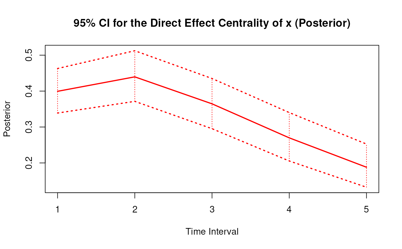
#> 1 x 1 0.3993 0.0335 1000 0.3295 0.4642
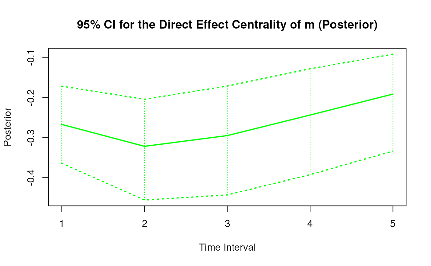
#> 2 m 1 -0.2662 0.0528 1000 -0.3760 -0.1607
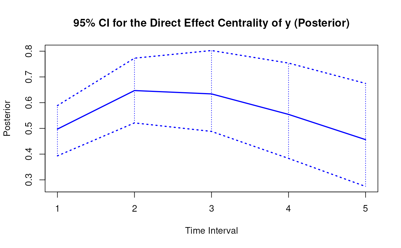
#> 3 y 1 0.4984 0.0523 1000 0.3935 0.5975
#> 4 x 2 0.4399 0.0383 1000 0.3635 0.5180
#> 5 m 2 -0.3206 0.0683 1000 -0.4639 -0.1916
#> 6 y 2 0.6495 0.0682 1000 0.5172 0.7789
#> 7 x 3 0.3650 0.0383 1000 0.2953 0.4459
#> 8 m 3 -0.2937 0.0720 1000 -0.4458 -0.1649
#> 9 y 3 0.6384 0.0829 1000 0.4855 0.7960
#> 10 x 4 0.2703 0.0360 1000 0.2074 0.3468
#> 11 m 4 -0.2424 0.0705 1000 -0.3955 -0.1253
#> 12 y 4 0.5606 0.0965 1000 0.3886 0.7494
#> 13 x 5 0.1885 0.0319 1000 0.1347 0.2548
#> 14 m 5 -0.1902 0.0661 1000 -0.3391 -0.0873
#> 15 y 5 0.4640 0.1061 1000 0.2800 0.6815
summary(posterior)
#> Call:
#> PosteriorDirectCentral(phi = phi, delta_t = 1:5)
#>
#> Direct Effect Centrality
#> variable interval est se R 2.5% 97.5%
#> 1 x 1 0.3993 0.0335 1000 0.3295 0.4642
#> 2 m 1 -0.2662 0.0528 1000 -0.3760 -0.1607
#> 3 y 1 0.4984 0.0523 1000 0.3935 0.5975
#> 4 x 2 0.4399 0.0383 1000 0.3635 0.5180
#> 5 m 2 -0.3206 0.0683 1000 -0.4639 -0.1916
#> 6 y 2 0.6495 0.0682 1000 0.5172 0.7789
#> 7 x 3 0.3650 0.0383 1000 0.2953 0.4459
#> 8 m 3 -0.2937 0.0720 1000 -0.4458 -0.1649
#> 9 y 3 0.6384 0.0829 1000 0.4855 0.7960
#> 10 x 4 0.2703 0.0360 1000 0.2074 0.3468
#> 11 m 4 -0.2424 0.0705 1000 -0.3955 -0.1253
#> 12 y 4 0.5606 0.0965 1000 0.3886 0.7494
#> 13 x 5 0.1885 0.0319 1000 0.1347 0.2548
#> 14 m 5 -0.1902 0.0661 1000 -0.3391 -0.0873
#> 15 y 5 0.4640 0.1061 1000 0.2800 0.6815
confint(posterior, level = 0.95)
#> variable interval 2.5 % 97.5 %
#> 1 x 1 0.3294530 0.46424832
#> 2 m 1 -0.3759764 -0.16068352
#> 3 y 1 0.3934741 0.59750623
#> 4 x 2 0.3634918 0.51800595
#> 5 m 2 -0.4638899 -0.19155180
#> 6 y 2 0.5171542 0.77891594
#> 7 x 3 0.2952871 0.44594783
#> 8 m 3 -0.4457505 -0.16494913
#> 9 y 3 0.4854694 0.79596015
#> 10 x 4 0.2074397 0.34678349
#> 11 m 4 -0.3955130 -0.12531371
#> 12 y 4 0.3885645 0.74935306
#> 13 x 5 0.1346536 0.25478865
#> 14 m 5 -0.3390776 -0.08731607
#> 15 y 5 0.2799563 0.68147463
plot(posterior)