Posterior Distribution for the Elements of the Standardized Matrix of Lagged Coefficients Over a Specific Time Interval or a Range of Time Intervals
Source:R/cTMed-posterior-beta-std.R
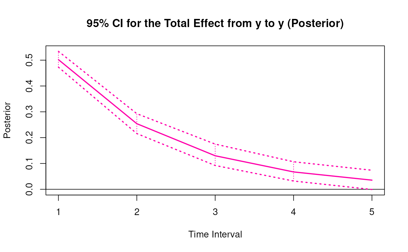
PosteriorBetaStd.RdThis function generates a posterior distribution for the elements of the standardized matrix of lagged coefficients \(\boldsymbol{\beta}\) over a specific time interval \(\Delta t\) or a range of time intervals using the posterior distribution of the first-order stochastic differential equation model drift matrix \(\boldsymbol{\Phi}\) and process noise covariance matrix \(\boldsymbol{\Sigma}\).
Arguments
- phi
List of numeric matrices. Each element of the list is a sample from the posterior distribution of the drift matrix (\(\boldsymbol{\Phi}\)). Each matrix should have row and column names pertaining to the variables in the system.
- sigma
List of numeric matrices. Each element of the list is a sample from the posterior distribution of the process noise covariance matrix (\(\boldsymbol{\Sigma}\)). Each matrix should have row and column names pertaining to the variables in the system.
- delta_t
Numeric. Time interval (\(\Delta t\)).
- ncores
Positive integer. Number of cores to use. If
ncores = NULL, use a single core. Consider using multiple cores when number of replicationsRis a large value.- tol
Numeric. Smallest possible time interval to allow.
Value
Returns an object
of class ctmedmc which is a list with the following elements:
- call
Function call.
- args
Function arguments.
- fun
Function used ("PosteriorBetaStd").
- output
A list of length
length(delta_t).
Each element in the output list has the following elements:
- est
Mean of the posterior distribution of the elements of the standardized matrix of lagged coefficients.
- thetahatstar
Posterior distribution of the elements of the standardized matrix of lagged coefficients.
Details
See TotalStd() for more details.
References
Bollen, K. A. (1987). Total, direct, and indirect effects in structural equation models. Sociological Methodology, 17, 37. doi:10.2307/271028
Deboeck, P. R., & Preacher, K. J. (2015). No need to be discrete: A method for continuous time mediation analysis. Structural Equation Modeling: A Multidisciplinary Journal, 23 (1), 61-75. doi:10.1080/10705511.2014.973960
Pesigan, I. J. A., Russell, M. A., & Chow, S.-M. (2025). Inferences and effect sizes for direct, indirect, and total effects in continuous-time mediation models. Psychological Methods. doi:10.1037/met0000779
Ryan, O., & Hamaker, E. L. (2021). Time to intervene: A continuous-time approach to network analysis and centrality. Psychometrika, 87 (1), 214-252. doi:10.1007/s11336-021-09767-0
See also
Other Continuous-Time Mediation Functions:
BootBeta(),
BootBetaStd(),
BootDirectCentral(),
BootDirectCentralStd(),
BootIndirectCentral(),
BootIndirectCentralStd(),
BootMed(),
BootMedStd(),
BootTotalCentral(),
BootTotalCentralStd(),
DeltaBeta(),
DeltaBetaStd(),
DeltaDirectCentral(),
DeltaDirectCentralStd(),
DeltaIndirectCentral(),
DeltaMed(),
DeltaMedStd(),
DeltaTotalCentral(),
DeltaTotalCentralStd(),
Direct(),
DirectCentral(),
DirectCentralStd(),
DirectStd(),
Indirect(),
IndirectCentral(),
IndirectCentralStd(),
IndirectStd(),
MCBeta(),
MCBetaStd(),
MCDirectCentral(),
MCDirectCentralStd(),
MCIndirectCentral(),
MCIndirectCentralStd(),
MCMed(),
MCMedStd(),
MCPhi(),
MCPhiSigma(),
MCTotalCentral(),
MCTotalCentralStd(),
Med(),
MedStd(),
PosteriorBeta(),
PosteriorDirectCentral(),
PosteriorDirectCentralStd(),
PosteriorIndirectCentral(),
PosteriorIndirectCentralStd(),
PosteriorMed(),
PosteriorMedStd(),
PosteriorTotalCentral(),
PosteriorTotalCentralStd(),
Total(),
TotalCentral(),
TotalCentralStd(),
TotalStd(),
Trajectory()
Examples
set.seed(42)
phi <- matrix(
data = c(
-0.357, 0.771, -0.450,
0.000, -0.511, 0.729,
0.000, 0.000, -0.693
),
nrow = 3
)
colnames(phi) <- rownames(phi) <- c("x", "m", "y")
sigma <- matrix(
data = c(
0.24455556, 0.02201587, -0.05004762,
0.02201587, 0.07067800, 0.01539456,
-0.05004762, 0.01539456, 0.07553061
),
nrow = 3
)
colnames(sigma) <- rownames(sigma) <- c("x", "m", "y")
input <- MCPhiSigma(
phi = phi,
sigma = sigma,
vcov_theta = 0.001 * diag(15),
R = 100L,
seed = 42
)$output
phi <- lapply(
X = input,
FUN = function(x) {
x[[1]]
}
)
sigma <- lapply(
X = input,
FUN = function(x) {
x[[2]]
}
)
# Specific time interval ----------------------------------------------------
PosteriorBetaStd(
phi = phi,
sigma = sigma,
delta_t = 1
)
#> Call:
#> PosteriorBetaStd(phi = phi, sigma = sigma, delta_t = 1)
#>
#> Total, Direct, and Indirect Effects
#>
#> effect interval est se R 2.5% 97.5%
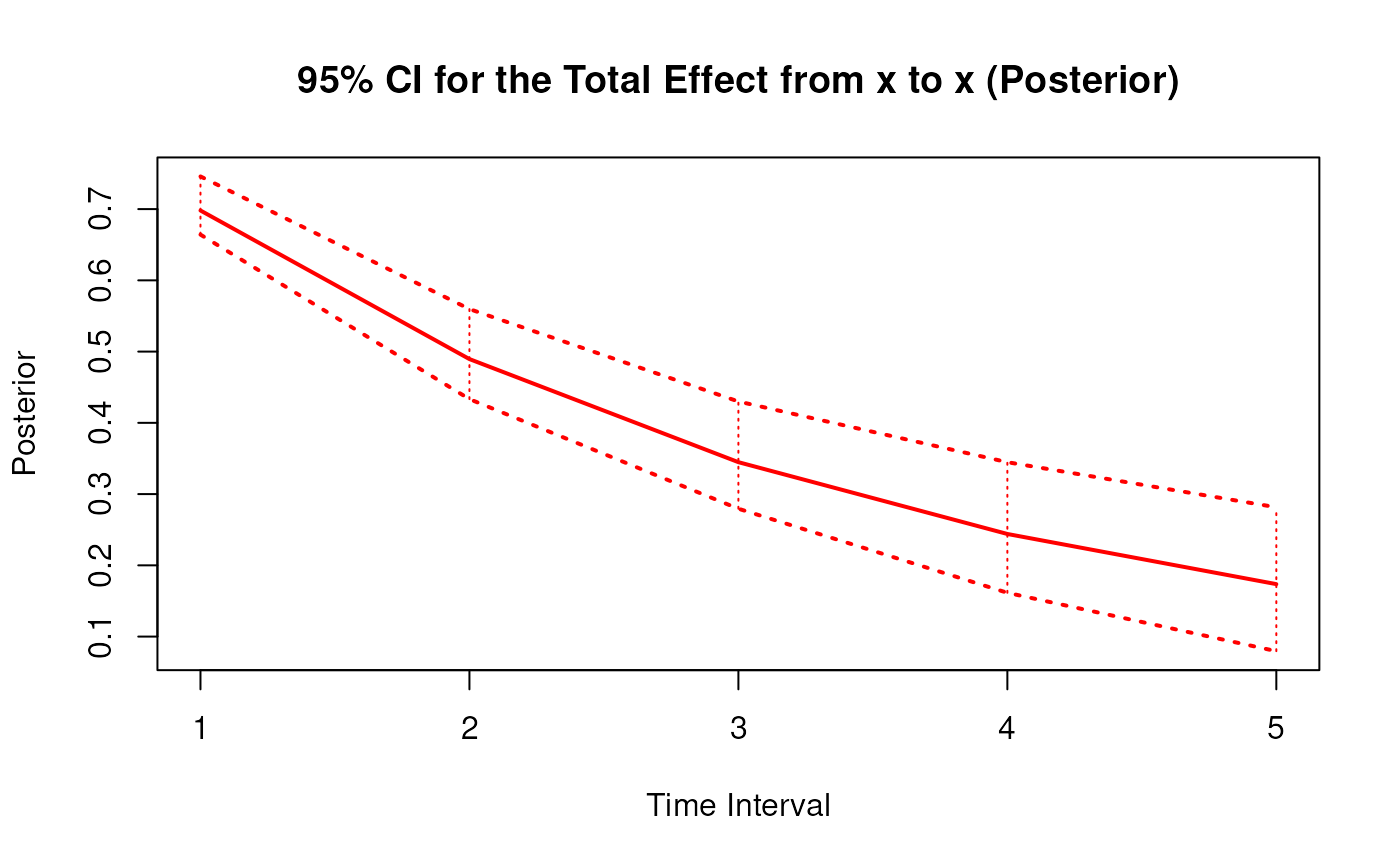
#> 1 from x to x 1 0.6980 0.0218 100 0.6642 0.7459
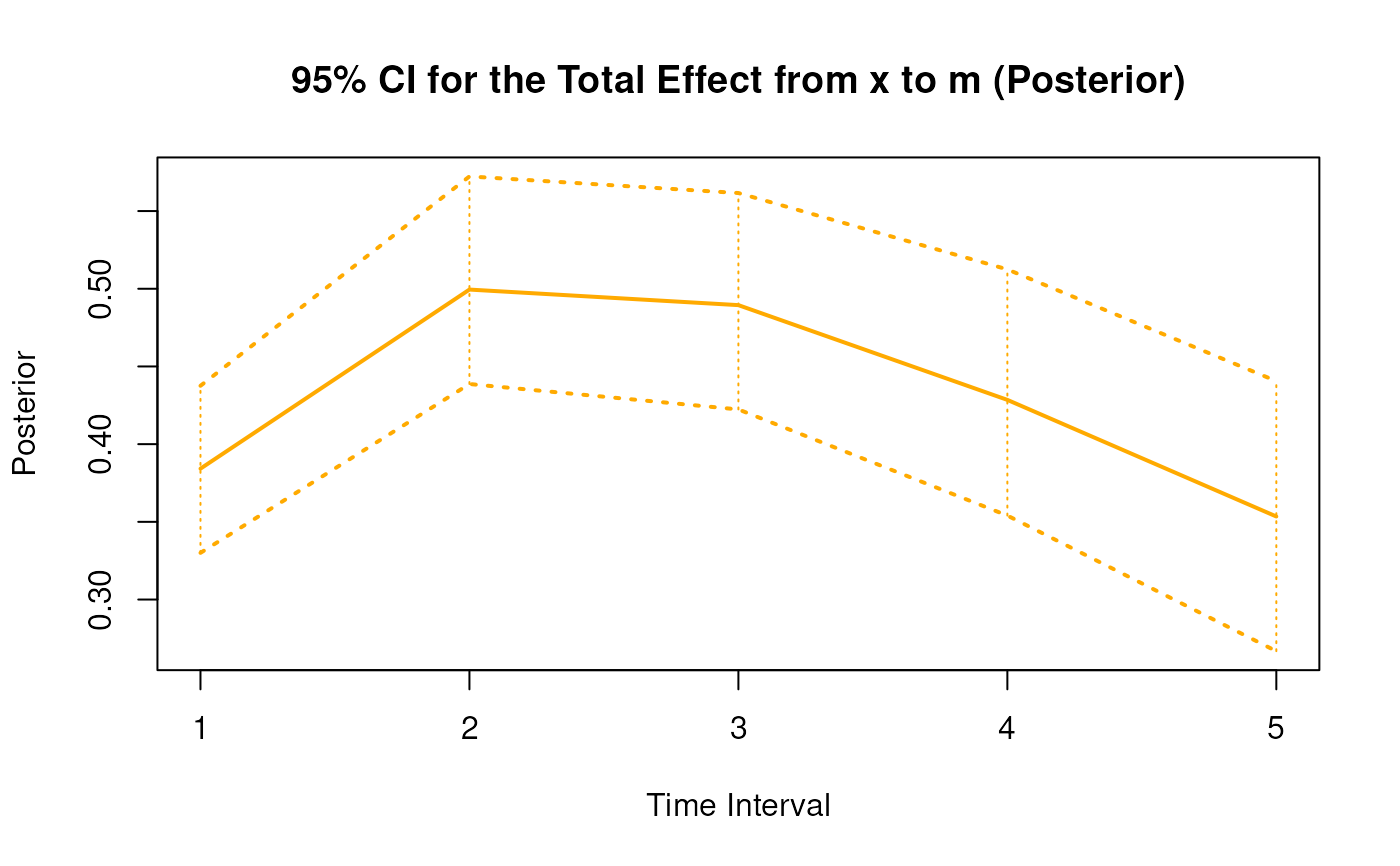
#> 2 from x to m 1 0.3842 0.0273 100 0.3300 0.4376
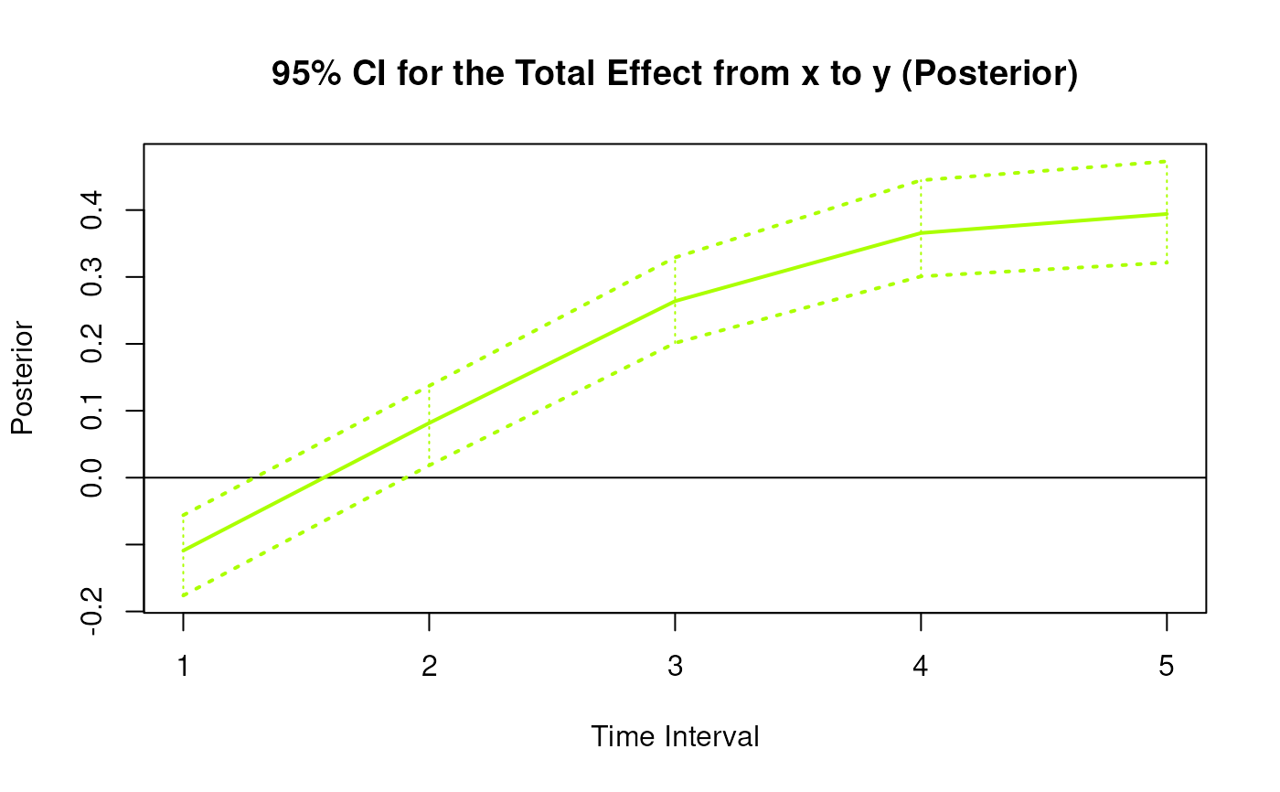
#> 3 from x to y 1 -0.1090 0.0310 100 -0.1762 -0.0561
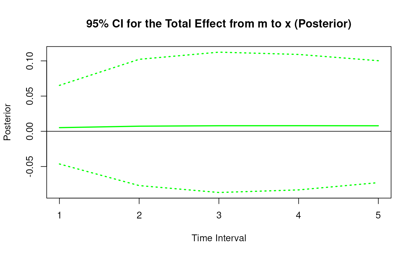
#> 4 from m to x 1 0.0052 0.0294 100 -0.0464 0.0652
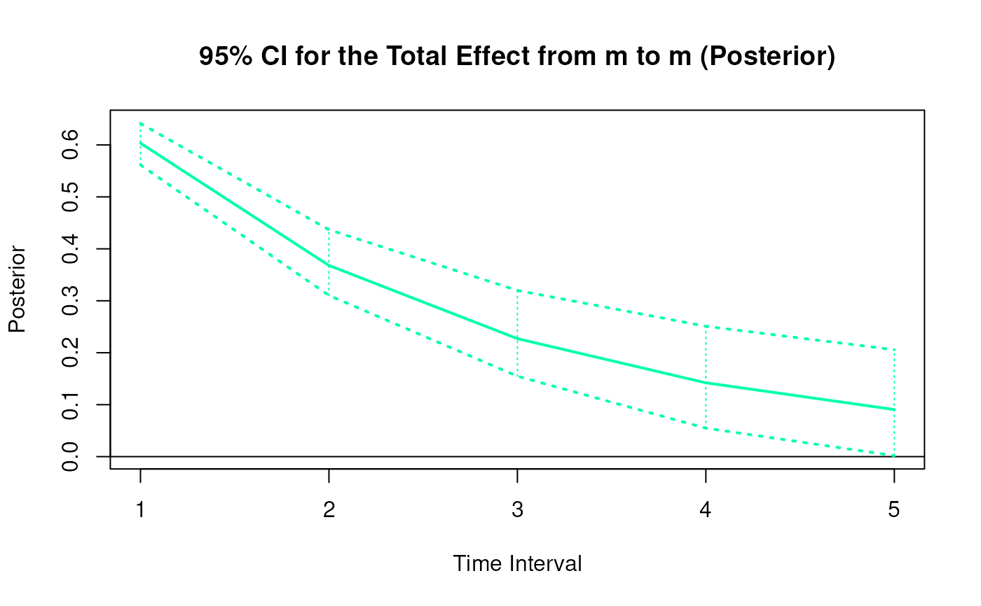
#> 5 from m to m 1 0.6034 0.0209 100 0.5615 0.6413
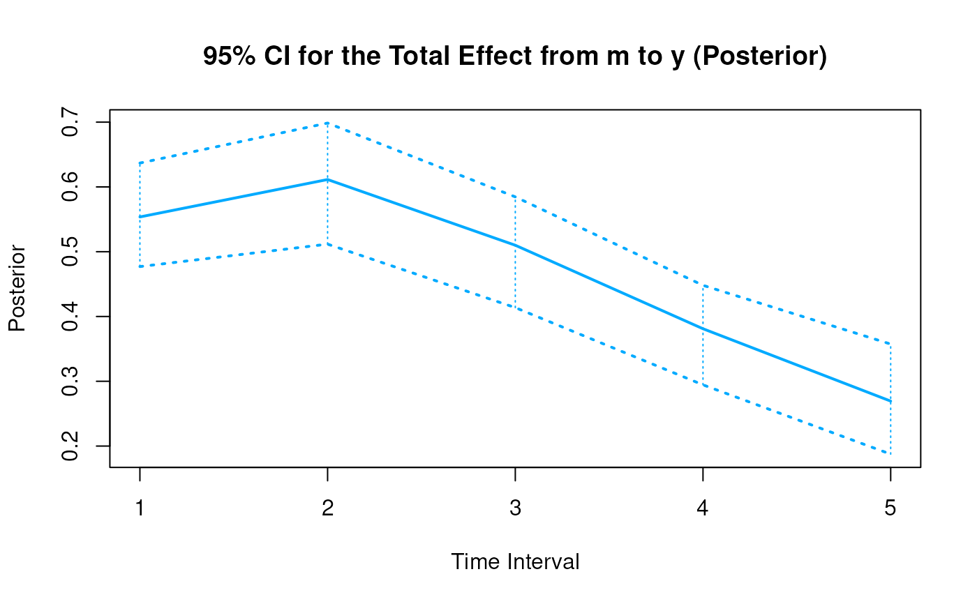
#> 6 from m to y 1 0.5537 0.0415 100 0.4770 0.6368
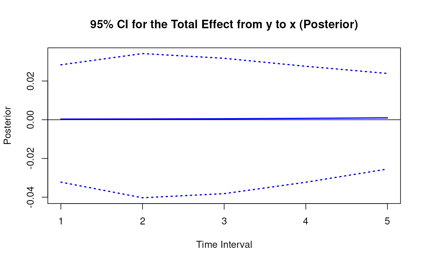
#> 7 from y to x 1 0.0003 0.0186 100 -0.0322 0.0284
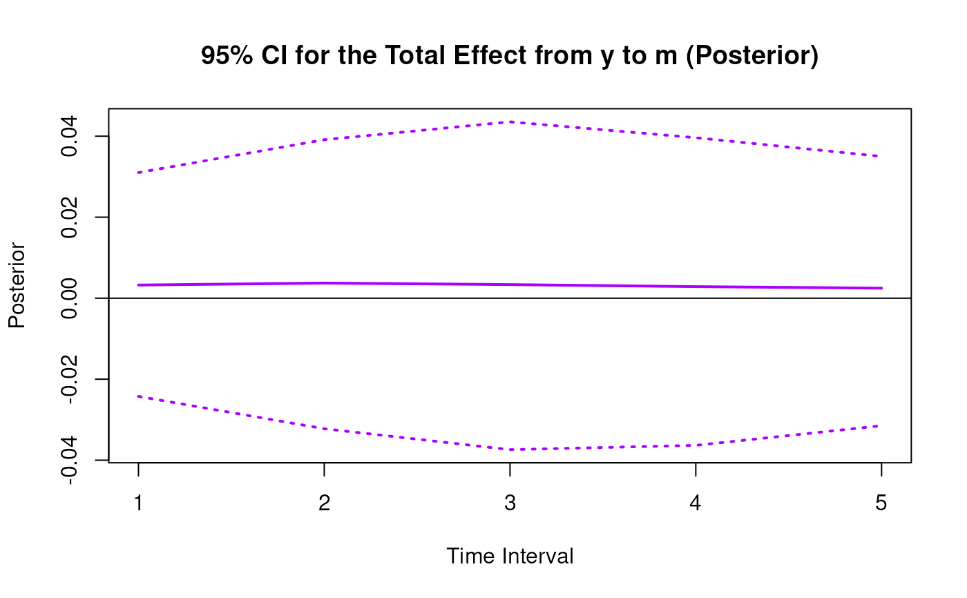
#> 8 from y to m 1 0.0032 0.0148 100 -0.0242 0.0310
#> 9 from y to y 1 0.5021 0.0158 100 0.4729 0.5342
# Range of time intervals ---------------------------------------------------
posterior <- PosteriorBetaStd(
phi = phi,
sigma = sigma,
delta_t = 1:5
)
plot(posterior)


 # Methods -------------------------------------------------------------------
# PosteriorBetaStd has a number of methods including
# print, summary, confint, and plot
print(posterior)
#> Call:
#> PosteriorBetaStd(phi = phi, sigma = sigma, delta_t = 1:5)
#>
#> Total, Direct, and Indirect Effects
#>
#> effect interval est se R 2.5% 97.5%
#> 1 from x to x 1 0.6980 0.0218 100 0.6642 0.7459
#> 2 from x to m 1 0.3842 0.0273 100 0.3300 0.4376
#> 3 from x to y 1 -0.1090 0.0310 100 -0.1762 -0.0561
#> 4 from m to x 1 0.0052 0.0294 100 -0.0464 0.0652
#> 5 from m to m 1 0.6034 0.0209 100 0.5615 0.6413
#> 6 from m to y 1 0.5537 0.0415 100 0.4770 0.6368
#> 7 from y to x 1 0.0003 0.0186 100 -0.0322 0.0284
#> 8 from y to m 1 0.0032 0.0148 100 -0.0242 0.0310
#> 9 from y to y 1 0.5021 0.0158 100 0.4729 0.5342
#> 10 from x to x 2 0.4895 0.0337 100 0.4333 0.5597
#> 11 from x to m 2 0.4995 0.0347 100 0.4387 0.5723
#> 12 from x to y 2 0.0817 0.0308 100 0.0184 0.1372
#> 13 from m to x 2 0.0073 0.0449 100 -0.0771 0.1022
#> 14 from m to m 2 0.3680 0.0348 100 0.3103 0.4368
#> 15 from m to y 2 0.6114 0.0466 100 0.5117 0.6986
#> 16 from y to x 2 0.0004 0.0225 100 -0.0403 0.0342
#> 17 from y to m 2 0.0037 0.0205 100 -0.0322 0.0391
#> 18 from y to y 2 0.2541 0.0202 100 0.2158 0.2928
#> 19 from x to x 3 0.3448 0.0413 100 0.2795 0.4300
#> 20 from x to m 3 0.4895 0.0373 100 0.4223 0.5616
#> 21 from x to y 3 0.2639 0.0329 100 0.2013 0.3291
#> 22 from m to x 3 0.0079 0.0507 100 -0.0869 0.1124
#> 23 from m to m 3 0.2271 0.0455 100 0.1548 0.3200
#> 24 from m to y 3 0.5100 0.0442 100 0.4137 0.5846
#> 25 from y to x 3 0.0005 0.0207 100 -0.0382 0.0317
#> 26 from y to m 3 0.0034 0.0226 100 -0.0374 0.0435
#> 27 from y to y 3 0.1299 0.0206 100 0.0922 0.1750
#> 28 from x to x 4 0.2440 0.0464 100 0.1615 0.3448
#> 29 from x to m 4 0.4285 0.0408 100 0.3540 0.5125
#> 30 from x to y 4 0.3657 0.0374 100 0.3009 0.4446
#> 31 from m to x 4 0.0080 0.0500 100 -0.0832 0.1091
#> 32 from m to m 4 0.1421 0.0519 100 0.0548 0.2509
#> 33 from m to y 4 0.3811 0.0435 100 0.2945 0.4481
#> 34 from y to x 4 0.0007 0.0173 100 -0.0323 0.0276
#> 35 from y to m 4 0.0029 0.0223 100 -0.0363 0.0396
#> 36 from y to y 4 0.0672 0.0203 100 0.0320 0.1066
#> 37 from x to x 5 0.1736 0.0493 100 0.0795 0.2815
#> 38 from x to m 5 0.3535 0.0457 100 0.2668 0.4406
#> 39 from x to y 5 0.3942 0.0416 100 0.3214 0.4728
#> 40 from m to x 5 0.0079 0.0457 100 -0.0729 0.1002
#> 41 from m to m 5 0.0906 0.0540 100 0.0019 0.2057
#> 42 from m to y 5 0.2694 0.0453 100 0.1875 0.3574
#> 43 from y to x 5 0.0010 0.0137 100 -0.0255 0.0239
#> 44 from y to m 5 0.0025 0.0205 100 -0.0315 0.0350
#> 45 from y to y 5 0.0354 0.0201 100 -0.0007 0.0738
summary(posterior)
#> Call:
#> PosteriorBetaStd(phi = phi, sigma = sigma, delta_t = 1:5)
#>
#> Total, Direct, and Indirect Effects
#>
#> effect interval est se R 2.5% 97.5%
#> 1 from x to x 1 0.6980 0.0218 100 0.6642 0.7459
#> 2 from x to m 1 0.3842 0.0273 100 0.3300 0.4376
#> 3 from x to y 1 -0.1090 0.0310 100 -0.1762 -0.0561
#> 4 from m to x 1 0.0052 0.0294 100 -0.0464 0.0652
#> 5 from m to m 1 0.6034 0.0209 100 0.5615 0.6413
#> 6 from m to y 1 0.5537 0.0415 100 0.4770 0.6368
#> 7 from y to x 1 0.0003 0.0186 100 -0.0322 0.0284
#> 8 from y to m 1 0.0032 0.0148 100 -0.0242 0.0310
#> 9 from y to y 1 0.5021 0.0158 100 0.4729 0.5342
#> 10 from x to x 2 0.4895 0.0337 100 0.4333 0.5597
#> 11 from x to m 2 0.4995 0.0347 100 0.4387 0.5723
#> 12 from x to y 2 0.0817 0.0308 100 0.0184 0.1372
#> 13 from m to x 2 0.0073 0.0449 100 -0.0771 0.1022
#> 14 from m to m 2 0.3680 0.0348 100 0.3103 0.4368
#> 15 from m to y 2 0.6114 0.0466 100 0.5117 0.6986
#> 16 from y to x 2 0.0004 0.0225 100 -0.0403 0.0342
#> 17 from y to m 2 0.0037 0.0205 100 -0.0322 0.0391
#> 18 from y to y 2 0.2541 0.0202 100 0.2158 0.2928
#> 19 from x to x 3 0.3448 0.0413 100 0.2795 0.4300
#> 20 from x to m 3 0.4895 0.0373 100 0.4223 0.5616
#> 21 from x to y 3 0.2639 0.0329 100 0.2013 0.3291
#> 22 from m to x 3 0.0079 0.0507 100 -0.0869 0.1124
#> 23 from m to m 3 0.2271 0.0455 100 0.1548 0.3200
#> 24 from m to y 3 0.5100 0.0442 100 0.4137 0.5846
#> 25 from y to x 3 0.0005 0.0207 100 -0.0382 0.0317
#> 26 from y to m 3 0.0034 0.0226 100 -0.0374 0.0435
#> 27 from y to y 3 0.1299 0.0206 100 0.0922 0.1750
#> 28 from x to x 4 0.2440 0.0464 100 0.1615 0.3448
#> 29 from x to m 4 0.4285 0.0408 100 0.3540 0.5125
#> 30 from x to y 4 0.3657 0.0374 100 0.3009 0.4446
#> 31 from m to x 4 0.0080 0.0500 100 -0.0832 0.1091
#> 32 from m to m 4 0.1421 0.0519 100 0.0548 0.2509
#> 33 from m to y 4 0.3811 0.0435 100 0.2945 0.4481
#> 34 from y to x 4 0.0007 0.0173 100 -0.0323 0.0276
#> 35 from y to m 4 0.0029 0.0223 100 -0.0363 0.0396
#> 36 from y to y 4 0.0672 0.0203 100 0.0320 0.1066
#> 37 from x to x 5 0.1736 0.0493 100 0.0795 0.2815
#> 38 from x to m 5 0.3535 0.0457 100 0.2668 0.4406
#> 39 from x to y 5 0.3942 0.0416 100 0.3214 0.4728
#> 40 from m to x 5 0.0079 0.0457 100 -0.0729 0.1002
#> 41 from m to m 5 0.0906 0.0540 100 0.0019 0.2057
#> 42 from m to y 5 0.2694 0.0453 100 0.1875 0.3574
#> 43 from y to x 5 0.0010 0.0137 100 -0.0255 0.0239
#> 44 from y to m 5 0.0025 0.0205 100 -0.0315 0.0350
#> 45 from y to y 5 0.0354 0.0201 100 -0.0007 0.0738
confint(posterior, level = 0.95)
#> effect interval 2.5 % 97.5 %
#> 1 from x to x 1 0.6641749590 0.74585310
#> 2 from x to m 1 0.3300370135 0.43755594
#> 3 from x to y 1 -0.1761840465 -0.05608631
#> 4 from m to x 1 -0.0464039176 0.06519135
#> 5 from m to m 1 0.5614760443 0.64133202
#> 6 from m to y 1 0.4770205167 0.63681685
#> 7 from y to x 1 -0.0322230255 0.02837078
#> 8 from y to m 1 -0.0242474280 0.03102154
#> 9 from y to y 1 0.4728679816 0.53416076
#> 10 from x to x 2 0.4332999182 0.55968990
#> 11 from x to m 2 0.4387006578 0.57228591
#> 12 from x to y 2 0.0183512271 0.13718923
#> 13 from m to x 2 -0.0770755264 0.10222351
#> 14 from m to m 2 0.3103273900 0.43684113
#> 15 from m to y 2 0.5116559371 0.69857736
#> 16 from y to x 2 -0.0402952378 0.03416504
#> 17 from y to m 2 -0.0322358248 0.03913211
#> 18 from y to y 2 0.2157841819 0.29280935
#> 19 from x to x 3 0.2794531041 0.42997191
#> 20 from x to m 3 0.4223455095 0.56160368
#> 21 from x to y 3 0.2013171762 0.32912929
#> 22 from m to x 3 -0.0868924433 0.11238272
#> 23 from m to m 3 0.1548158417 0.31996575
#> 24 from m to y 3 0.4136912017 0.58463038
#> 25 from y to x 3 -0.0381694773 0.03172716
#> 26 from y to m 3 -0.0373980327 0.04354727
#> 27 from y to y 3 0.0922332351 0.17499544
#> 28 from x to x 4 0.1614720669 0.34475219
#> 29 from x to m 4 0.3540402587 0.51246188
#> 30 from x to y 4 0.3008914033 0.44455601
#> 31 from m to x 4 -0.0832006827 0.10913370
#> 32 from m to m 4 0.0547795045 0.25093190
#> 33 from m to y 4 0.2944818859 0.44811038
#> 34 from y to x 4 -0.0322825095 0.02760479
#> 35 from y to m 4 -0.0363350603 0.03962832
#> 36 from y to y 4 0.0320274558 0.10661204
#> 37 from x to x 5 0.0795303141 0.28152308
#> 38 from x to m 5 0.2667744460 0.44057367
#> 39 from x to y 5 0.3214114308 0.47281052
#> 40 from m to x 5 -0.0728863312 0.10022551
#> 41 from m to m 5 0.0018636081 0.20573242
#> 42 from m to y 5 0.1874892609 0.35739944
#> 43 from y to x 5 -0.0254587018 0.02389312
#> 44 from y to m 5 -0.0314856711 0.03500352
#> 45 from y to y 5 -0.0007345249 0.07379267
plot(posterior)
# Methods -------------------------------------------------------------------
# PosteriorBetaStd has a number of methods including
# print, summary, confint, and plot
print(posterior)
#> Call:
#> PosteriorBetaStd(phi = phi, sigma = sigma, delta_t = 1:5)
#>
#> Total, Direct, and Indirect Effects
#>
#> effect interval est se R 2.5% 97.5%
#> 1 from x to x 1 0.6980 0.0218 100 0.6642 0.7459
#> 2 from x to m 1 0.3842 0.0273 100 0.3300 0.4376
#> 3 from x to y 1 -0.1090 0.0310 100 -0.1762 -0.0561
#> 4 from m to x 1 0.0052 0.0294 100 -0.0464 0.0652
#> 5 from m to m 1 0.6034 0.0209 100 0.5615 0.6413
#> 6 from m to y 1 0.5537 0.0415 100 0.4770 0.6368
#> 7 from y to x 1 0.0003 0.0186 100 -0.0322 0.0284
#> 8 from y to m 1 0.0032 0.0148 100 -0.0242 0.0310
#> 9 from y to y 1 0.5021 0.0158 100 0.4729 0.5342
#> 10 from x to x 2 0.4895 0.0337 100 0.4333 0.5597
#> 11 from x to m 2 0.4995 0.0347 100 0.4387 0.5723
#> 12 from x to y 2 0.0817 0.0308 100 0.0184 0.1372
#> 13 from m to x 2 0.0073 0.0449 100 -0.0771 0.1022
#> 14 from m to m 2 0.3680 0.0348 100 0.3103 0.4368
#> 15 from m to y 2 0.6114 0.0466 100 0.5117 0.6986
#> 16 from y to x 2 0.0004 0.0225 100 -0.0403 0.0342
#> 17 from y to m 2 0.0037 0.0205 100 -0.0322 0.0391
#> 18 from y to y 2 0.2541 0.0202 100 0.2158 0.2928
#> 19 from x to x 3 0.3448 0.0413 100 0.2795 0.4300
#> 20 from x to m 3 0.4895 0.0373 100 0.4223 0.5616
#> 21 from x to y 3 0.2639 0.0329 100 0.2013 0.3291
#> 22 from m to x 3 0.0079 0.0507 100 -0.0869 0.1124
#> 23 from m to m 3 0.2271 0.0455 100 0.1548 0.3200
#> 24 from m to y 3 0.5100 0.0442 100 0.4137 0.5846
#> 25 from y to x 3 0.0005 0.0207 100 -0.0382 0.0317
#> 26 from y to m 3 0.0034 0.0226 100 -0.0374 0.0435
#> 27 from y to y 3 0.1299 0.0206 100 0.0922 0.1750
#> 28 from x to x 4 0.2440 0.0464 100 0.1615 0.3448
#> 29 from x to m 4 0.4285 0.0408 100 0.3540 0.5125
#> 30 from x to y 4 0.3657 0.0374 100 0.3009 0.4446
#> 31 from m to x 4 0.0080 0.0500 100 -0.0832 0.1091
#> 32 from m to m 4 0.1421 0.0519 100 0.0548 0.2509
#> 33 from m to y 4 0.3811 0.0435 100 0.2945 0.4481
#> 34 from y to x 4 0.0007 0.0173 100 -0.0323 0.0276
#> 35 from y to m 4 0.0029 0.0223 100 -0.0363 0.0396
#> 36 from y to y 4 0.0672 0.0203 100 0.0320 0.1066
#> 37 from x to x 5 0.1736 0.0493 100 0.0795 0.2815
#> 38 from x to m 5 0.3535 0.0457 100 0.2668 0.4406
#> 39 from x to y 5 0.3942 0.0416 100 0.3214 0.4728
#> 40 from m to x 5 0.0079 0.0457 100 -0.0729 0.1002
#> 41 from m to m 5 0.0906 0.0540 100 0.0019 0.2057
#> 42 from m to y 5 0.2694 0.0453 100 0.1875 0.3574
#> 43 from y to x 5 0.0010 0.0137 100 -0.0255 0.0239
#> 44 from y to m 5 0.0025 0.0205 100 -0.0315 0.0350
#> 45 from y to y 5 0.0354 0.0201 100 -0.0007 0.0738
summary(posterior)
#> Call:
#> PosteriorBetaStd(phi = phi, sigma = sigma, delta_t = 1:5)
#>
#> Total, Direct, and Indirect Effects
#>
#> effect interval est se R 2.5% 97.5%
#> 1 from x to x 1 0.6980 0.0218 100 0.6642 0.7459
#> 2 from x to m 1 0.3842 0.0273 100 0.3300 0.4376
#> 3 from x to y 1 -0.1090 0.0310 100 -0.1762 -0.0561
#> 4 from m to x 1 0.0052 0.0294 100 -0.0464 0.0652
#> 5 from m to m 1 0.6034 0.0209 100 0.5615 0.6413
#> 6 from m to y 1 0.5537 0.0415 100 0.4770 0.6368
#> 7 from y to x 1 0.0003 0.0186 100 -0.0322 0.0284
#> 8 from y to m 1 0.0032 0.0148 100 -0.0242 0.0310
#> 9 from y to y 1 0.5021 0.0158 100 0.4729 0.5342
#> 10 from x to x 2 0.4895 0.0337 100 0.4333 0.5597
#> 11 from x to m 2 0.4995 0.0347 100 0.4387 0.5723
#> 12 from x to y 2 0.0817 0.0308 100 0.0184 0.1372
#> 13 from m to x 2 0.0073 0.0449 100 -0.0771 0.1022
#> 14 from m to m 2 0.3680 0.0348 100 0.3103 0.4368
#> 15 from m to y 2 0.6114 0.0466 100 0.5117 0.6986
#> 16 from y to x 2 0.0004 0.0225 100 -0.0403 0.0342
#> 17 from y to m 2 0.0037 0.0205 100 -0.0322 0.0391
#> 18 from y to y 2 0.2541 0.0202 100 0.2158 0.2928
#> 19 from x to x 3 0.3448 0.0413 100 0.2795 0.4300
#> 20 from x to m 3 0.4895 0.0373 100 0.4223 0.5616
#> 21 from x to y 3 0.2639 0.0329 100 0.2013 0.3291
#> 22 from m to x 3 0.0079 0.0507 100 -0.0869 0.1124
#> 23 from m to m 3 0.2271 0.0455 100 0.1548 0.3200
#> 24 from m to y 3 0.5100 0.0442 100 0.4137 0.5846
#> 25 from y to x 3 0.0005 0.0207 100 -0.0382 0.0317
#> 26 from y to m 3 0.0034 0.0226 100 -0.0374 0.0435
#> 27 from y to y 3 0.1299 0.0206 100 0.0922 0.1750
#> 28 from x to x 4 0.2440 0.0464 100 0.1615 0.3448
#> 29 from x to m 4 0.4285 0.0408 100 0.3540 0.5125
#> 30 from x to y 4 0.3657 0.0374 100 0.3009 0.4446
#> 31 from m to x 4 0.0080 0.0500 100 -0.0832 0.1091
#> 32 from m to m 4 0.1421 0.0519 100 0.0548 0.2509
#> 33 from m to y 4 0.3811 0.0435 100 0.2945 0.4481
#> 34 from y to x 4 0.0007 0.0173 100 -0.0323 0.0276
#> 35 from y to m 4 0.0029 0.0223 100 -0.0363 0.0396
#> 36 from y to y 4 0.0672 0.0203 100 0.0320 0.1066
#> 37 from x to x 5 0.1736 0.0493 100 0.0795 0.2815
#> 38 from x to m 5 0.3535 0.0457 100 0.2668 0.4406
#> 39 from x to y 5 0.3942 0.0416 100 0.3214 0.4728
#> 40 from m to x 5 0.0079 0.0457 100 -0.0729 0.1002
#> 41 from m to m 5 0.0906 0.0540 100 0.0019 0.2057
#> 42 from m to y 5 0.2694 0.0453 100 0.1875 0.3574
#> 43 from y to x 5 0.0010 0.0137 100 -0.0255 0.0239
#> 44 from y to m 5 0.0025 0.0205 100 -0.0315 0.0350
#> 45 from y to y 5 0.0354 0.0201 100 -0.0007 0.0738
confint(posterior, level = 0.95)
#> effect interval 2.5 % 97.5 %
#> 1 from x to x 1 0.6641749590 0.74585310
#> 2 from x to m 1 0.3300370135 0.43755594
#> 3 from x to y 1 -0.1761840465 -0.05608631
#> 4 from m to x 1 -0.0464039176 0.06519135
#> 5 from m to m 1 0.5614760443 0.64133202
#> 6 from m to y 1 0.4770205167 0.63681685
#> 7 from y to x 1 -0.0322230255 0.02837078
#> 8 from y to m 1 -0.0242474280 0.03102154
#> 9 from y to y 1 0.4728679816 0.53416076
#> 10 from x to x 2 0.4332999182 0.55968990
#> 11 from x to m 2 0.4387006578 0.57228591
#> 12 from x to y 2 0.0183512271 0.13718923
#> 13 from m to x 2 -0.0770755264 0.10222351
#> 14 from m to m 2 0.3103273900 0.43684113
#> 15 from m to y 2 0.5116559371 0.69857736
#> 16 from y to x 2 -0.0402952378 0.03416504
#> 17 from y to m 2 -0.0322358248 0.03913211
#> 18 from y to y 2 0.2157841819 0.29280935
#> 19 from x to x 3 0.2794531041 0.42997191
#> 20 from x to m 3 0.4223455095 0.56160368
#> 21 from x to y 3 0.2013171762 0.32912929
#> 22 from m to x 3 -0.0868924433 0.11238272
#> 23 from m to m 3 0.1548158417 0.31996575
#> 24 from m to y 3 0.4136912017 0.58463038
#> 25 from y to x 3 -0.0381694773 0.03172716
#> 26 from y to m 3 -0.0373980327 0.04354727
#> 27 from y to y 3 0.0922332351 0.17499544
#> 28 from x to x 4 0.1614720669 0.34475219
#> 29 from x to m 4 0.3540402587 0.51246188
#> 30 from x to y 4 0.3008914033 0.44455601
#> 31 from m to x 4 -0.0832006827 0.10913370
#> 32 from m to m 4 0.0547795045 0.25093190
#> 33 from m to y 4 0.2944818859 0.44811038
#> 34 from y to x 4 -0.0322825095 0.02760479
#> 35 from y to m 4 -0.0363350603 0.03962832
#> 36 from y to y 4 0.0320274558 0.10661204
#> 37 from x to x 5 0.0795303141 0.28152308
#> 38 from x to m 5 0.2667744460 0.44057367
#> 39 from x to y 5 0.3214114308 0.47281052
#> 40 from m to x 5 -0.0728863312 0.10022551
#> 41 from m to m 5 0.0018636081 0.20573242
#> 42 from m to y 5 0.1874892609 0.35739944
#> 43 from y to x 5 -0.0254587018 0.02389312
#> 44 from y to m 5 -0.0314856711 0.03500352
#> 45 from y to y 5 -0.0007345249 0.07379267
plot(posterior)