Posterior Distribution of Standardized Total, Direct, and Indirect Effects of X on Y Through M Over a Specific Time Interval or a Range of Time Intervals
Source:R/cTMed-posterior-med-std.R
PosteriorMedStd.RdThis function generates a posterior distribution of the standardized total, direct, and indirect effects of the independent variable \(X\) on the dependent variable \(Y\) through mediator variables \(\mathbf{m}\) over a specific time interval \(\Delta t\) or a range of time intervals using the posterior distribution of the first-order stochastic differential equation model drift matrix \(\boldsymbol{\Phi}\) and process noise covariance matrix \(\boldsymbol{\Sigma}\).
Arguments
- phi
List of numeric matrices. Each element of the list is a sample from the posterior distribution of the drift matrix (\(\boldsymbol{\Phi}\)). Each matrix should have row and column names pertaining to the variables in the system.
- sigma
List of numeric matrices. Each element of the list is a sample from the posterior distribution of the process noise covariance matrix (\(\boldsymbol{\Sigma}\)). Each matrix should have row and column names pertaining to the variables in the system.
- delta_t
Numeric. Time interval (\(\Delta t\)).
- from
Character string. Name of the independent variable \(X\) in
phi.- to
Character string. Name of the dependent variable \(Y\) in
phi.- med
Character vector. Name/s of the mediator variable/s in
phi.- ncores
Positive integer. Number of cores to use. If
ncores = NULL, use a single core. Consider using multiple cores when number of replicationsRis a large value.- tol
Numeric. Smallest possible time interval to allow.
Value
Returns an object
of class ctmedmc which is a list with the following elements:
- call
Function call.
- args
Function arguments.
- fun
Function used ("PosteriorMedStd").
- output
A list of length
length(delta_t).
Each element in the output list has the following elements:
- est
Mean of the posterior distribution of the standardized total, direct, and indirect effects.
- thetahatstar
Posterior distribution of the standardized total, direct, and indirect effects.
Details
See TotalStd(),
DirectStd(), and
IndirectStd() for more details.
References
Bollen, K. A. (1987). Total, direct, and indirect effects in structural equation models. Sociological Methodology, 17, 37. doi:10.2307/271028
Deboeck, P. R., & Preacher, K. J. (2015). No need to be discrete: A method for continuous time mediation analysis. Structural Equation Modeling: A Multidisciplinary Journal, 23 (1), 61-75. doi:10.1080/10705511.2014.973960
Pesigan, I. J. A., Russell, M. A., & Chow, S.-M. (2025). Inferences and effect sizes for direct, indirect, and total effects in continuous-time mediation models. Psychological Methods. doi:10.1037/met0000779
Ryan, O., & Hamaker, E. L. (2021). Time to intervene: A continuous-time approach to network analysis and centrality. Psychometrika, 87 (1), 214-252. doi:10.1007/s11336-021-09767-0
See also
Other Continuous-Time Mediation Functions:
BootBeta(),
BootBetaStd(),
BootDirectCentral(),
BootDirectCentralStd(),
BootIndirectCentral(),
BootIndirectCentralStd(),
BootMed(),
BootMedStd(),
BootTotalCentral(),
BootTotalCentralStd(),
DeltaBeta(),
DeltaBetaStd(),
DeltaDirectCentral(),
DeltaDirectCentralStd(),
DeltaIndirectCentral(),
DeltaMed(),
DeltaMedStd(),
DeltaTotalCentral(),
DeltaTotalCentralStd(),
Direct(),
DirectCentral(),
DirectCentralStd(),
DirectStd(),
Indirect(),
IndirectCentral(),
IndirectCentralStd(),
IndirectStd(),
MCBeta(),
MCBetaStd(),
MCDirectCentral(),
MCDirectCentralStd(),
MCIndirectCentral(),
MCIndirectCentralStd(),
MCMed(),
MCMedStd(),
MCPhi(),
MCPhiSigma(),
MCTotalCentral(),
MCTotalCentralStd(),
Med(),
MedStd(),
PosteriorBeta(),
PosteriorBetaStd(),
PosteriorDirectCentral(),
PosteriorDirectCentralStd(),
PosteriorIndirectCentral(),
PosteriorIndirectCentralStd(),
PosteriorMed(),
PosteriorTotalCentral(),
PosteriorTotalCentralStd(),
Total(),
TotalCentral(),
TotalCentralStd(),
TotalStd(),
Trajectory()
Examples
set.seed(42)
phi <- matrix(
data = c(
-0.357, 0.771, -0.450,
0.000, -0.511, 0.729,
0.000, 0.000, -0.693
),
nrow = 3
)
colnames(phi) <- rownames(phi) <- c("x", "m", "y")
sigma <- matrix(
data = c(
0.24455556, 0.02201587, -0.05004762,
0.02201587, 0.07067800, 0.01539456,
-0.05004762, 0.01539456, 0.07553061
),
nrow = 3
)
colnames(sigma) <- rownames(sigma) <- c("x", "m", "y")
input <- MCPhiSigma(
phi = phi,
sigma = sigma,
vcov_theta = 0.001 * diag(15),
R = 100L,
seed = 42
)$output
phi <- lapply(
X = input,
FUN = function(x) {
x[[1]]
}
)
sigma <- lapply(
X = input,
FUN = function(x) {
x[[2]]
}
)
# Specific time interval ----------------------------------------------------
PosteriorMedStd(
phi = phi,
sigma = sigma,
delta_t = 1,
from = "x",
to = "y",
med = "m"
)
#> Call:
#> PosteriorMedStd(phi = phi, sigma = sigma, delta_t = 1, from = "x",
#> to = "y", med = "m")
#>
#> Total, Direct, and Indirect Effects
#>
#> effect interval est se R 2.5% 97.5%
#> 1 total 1 -0.1090 0.0310 100 -0.1762 -0.0561
#> 2 direct 1 -0.2871 0.0447 100 -0.3931 -0.2081
#> 3 indirect 1 0.1781 0.0191 100 0.1450 0.2131
# Range of time intervals ---------------------------------------------------
posterior <- PosteriorMedStd(
phi = phi,
sigma = sigma,
delta_t = 1:5,
from = "x",
to = "y",
med = "m"
)
plot(posterior)

 # Methods -------------------------------------------------------------------
# PosteriorMedStd has a number of methods including
# print, summary, confint, and plot
print(posterior)
#> Call:
#> PosteriorMedStd(phi = phi, sigma = sigma, delta_t = 1:5, from = "x",
#> to = "y", med = "m")
#>
#> Total, Direct, and Indirect Effects
#>
#> effect interval est se R 2.5% 97.5%
#> 1 total 1 -0.1090 0.0310 100 -0.1762 -0.0561
#> 2 direct 1 -0.2871 0.0447 100 -0.3931 -0.2081
#> 3 indirect 1 0.1781 0.0191 100 0.1450 0.2131
#> 4 total 2 0.0817 0.0308 100 0.0184 0.1372
#> 5 direct 2 -0.3440 0.0560 100 -0.4782 -0.2484
#> 6 indirect 2 0.4257 0.0459 100 0.3526 0.5068
#> 7 total 3 0.2639 0.0329 100 0.2013 0.3291
#> 8 direct 3 -0.3122 0.0549 100 -0.4422 -0.2209
#> 9 indirect 3 0.5761 0.0642 100 0.4834 0.6927
#> 10 total 4 0.3657 0.0374 100 0.3009 0.4446
#> 11 direct 4 -0.2543 0.0496 100 -0.3685 -0.1760
#> 12 indirect 4 0.6200 0.0731 100 0.5112 0.7540
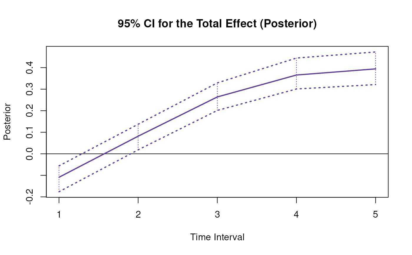
#> 13 total 5 0.3942 0.0416 100 0.3214 0.4728
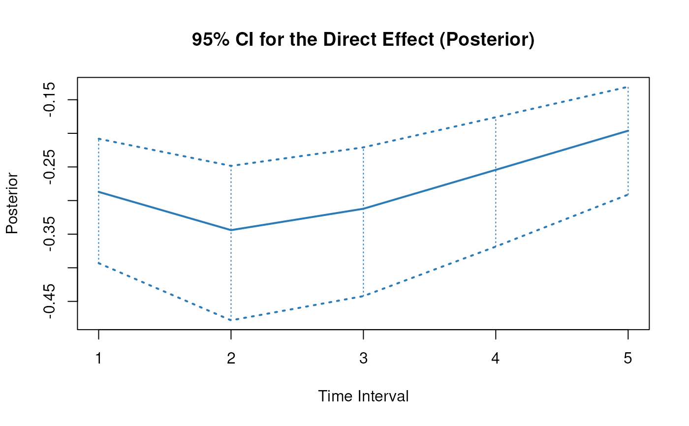
#> 14 direct 5 -0.1961 0.0433 100 -0.2911 -0.1308
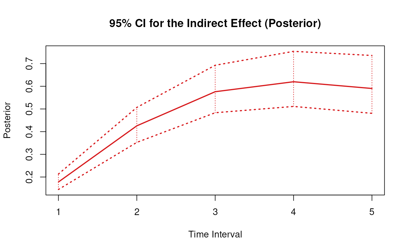
#> 15 indirect 5 0.5903 0.0752 100 0.4808 0.7358
summary(posterior)
#> Call:
#> PosteriorMedStd(phi = phi, sigma = sigma, delta_t = 1:5, from = "x",
#> to = "y", med = "m")
#>
#> Total, Direct, and Indirect Effects
#>
#> effect interval est se R 2.5% 97.5%
#> 1 total 1 -0.1090 0.0310 100 -0.1762 -0.0561
#> 2 direct 1 -0.2871 0.0447 100 -0.3931 -0.2081
#> 3 indirect 1 0.1781 0.0191 100 0.1450 0.2131
#> 4 total 2 0.0817 0.0308 100 0.0184 0.1372
#> 5 direct 2 -0.3440 0.0560 100 -0.4782 -0.2484
#> 6 indirect 2 0.4257 0.0459 100 0.3526 0.5068
#> 7 total 3 0.2639 0.0329 100 0.2013 0.3291
#> 8 direct 3 -0.3122 0.0549 100 -0.4422 -0.2209
#> 9 indirect 3 0.5761 0.0642 100 0.4834 0.6927
#> 10 total 4 0.3657 0.0374 100 0.3009 0.4446
#> 11 direct 4 -0.2543 0.0496 100 -0.3685 -0.1760
#> 12 indirect 4 0.6200 0.0731 100 0.5112 0.7540
#> 13 total 5 0.3942 0.0416 100 0.3214 0.4728
#> 14 direct 5 -0.1961 0.0433 100 -0.2911 -0.1308
#> 15 indirect 5 0.5903 0.0752 100 0.4808 0.7358
confint(posterior, level = 0.95)
#> effect interval 2.5 % 97.5 %
#> 1 total 1 -0.17618405 -0.05608631
#> 2 direct 1 -0.39314189 -0.20809131
#> 3 indirect 1 0.14504072 0.21309331
#> 4 total 2 0.01835123 0.13718923
#> 5 direct 2 -0.47816809 -0.24840869
#> 6 indirect 2 0.35262171 0.50678370
#> 7 total 3 0.20131718 0.32912929
#> 8 direct 3 -0.44216925 -0.22089823
#> 9 indirect 3 0.48340978 0.69268157
#> 10 total 4 0.30089140 0.44455601
#> 11 direct 4 -0.36848407 -0.17604808
#> 12 indirect 4 0.51116826 0.75404022
#> 13 total 5 0.32141143 0.47281052
#> 14 direct 5 -0.29110272 -0.13075872
#> 15 indirect 5 0.48079555 0.73583173
plot(posterior)
# Methods -------------------------------------------------------------------
# PosteriorMedStd has a number of methods including
# print, summary, confint, and plot
print(posterior)
#> Call:
#> PosteriorMedStd(phi = phi, sigma = sigma, delta_t = 1:5, from = "x",
#> to = "y", med = "m")
#>
#> Total, Direct, and Indirect Effects
#>
#> effect interval est se R 2.5% 97.5%
#> 1 total 1 -0.1090 0.0310 100 -0.1762 -0.0561
#> 2 direct 1 -0.2871 0.0447 100 -0.3931 -0.2081
#> 3 indirect 1 0.1781 0.0191 100 0.1450 0.2131
#> 4 total 2 0.0817 0.0308 100 0.0184 0.1372
#> 5 direct 2 -0.3440 0.0560 100 -0.4782 -0.2484
#> 6 indirect 2 0.4257 0.0459 100 0.3526 0.5068
#> 7 total 3 0.2639 0.0329 100 0.2013 0.3291
#> 8 direct 3 -0.3122 0.0549 100 -0.4422 -0.2209
#> 9 indirect 3 0.5761 0.0642 100 0.4834 0.6927
#> 10 total 4 0.3657 0.0374 100 0.3009 0.4446
#> 11 direct 4 -0.2543 0.0496 100 -0.3685 -0.1760
#> 12 indirect 4 0.6200 0.0731 100 0.5112 0.7540
#> 13 total 5 0.3942 0.0416 100 0.3214 0.4728
#> 14 direct 5 -0.1961 0.0433 100 -0.2911 -0.1308
#> 15 indirect 5 0.5903 0.0752 100 0.4808 0.7358
summary(posterior)
#> Call:
#> PosteriorMedStd(phi = phi, sigma = sigma, delta_t = 1:5, from = "x",
#> to = "y", med = "m")
#>
#> Total, Direct, and Indirect Effects
#>
#> effect interval est se R 2.5% 97.5%
#> 1 total 1 -0.1090 0.0310 100 -0.1762 -0.0561
#> 2 direct 1 -0.2871 0.0447 100 -0.3931 -0.2081
#> 3 indirect 1 0.1781 0.0191 100 0.1450 0.2131
#> 4 total 2 0.0817 0.0308 100 0.0184 0.1372
#> 5 direct 2 -0.3440 0.0560 100 -0.4782 -0.2484
#> 6 indirect 2 0.4257 0.0459 100 0.3526 0.5068
#> 7 total 3 0.2639 0.0329 100 0.2013 0.3291
#> 8 direct 3 -0.3122 0.0549 100 -0.4422 -0.2209
#> 9 indirect 3 0.5761 0.0642 100 0.4834 0.6927
#> 10 total 4 0.3657 0.0374 100 0.3009 0.4446
#> 11 direct 4 -0.2543 0.0496 100 -0.3685 -0.1760
#> 12 indirect 4 0.6200 0.0731 100 0.5112 0.7540
#> 13 total 5 0.3942 0.0416 100 0.3214 0.4728
#> 14 direct 5 -0.1961 0.0433 100 -0.2911 -0.1308
#> 15 indirect 5 0.5903 0.0752 100 0.4808 0.7358
confint(posterior, level = 0.95)
#> effect interval 2.5 % 97.5 %
#> 1 total 1 -0.17618405 -0.05608631
#> 2 direct 1 -0.39314189 -0.20809131
#> 3 indirect 1 0.14504072 0.21309331
#> 4 total 2 0.01835123 0.13718923
#> 5 direct 2 -0.47816809 -0.24840869
#> 6 indirect 2 0.35262171 0.50678370
#> 7 total 3 0.20131718 0.32912929
#> 8 direct 3 -0.44216925 -0.22089823
#> 9 indirect 3 0.48340978 0.69268157
#> 10 total 4 0.30089140 0.44455601
#> 11 direct 4 -0.36848407 -0.17604808
#> 12 indirect 4 0.51116826 0.75404022
#> 13 total 5 0.32141143 0.47281052
#> 14 direct 5 -0.29110272 -0.13075872
#> 15 indirect 5 0.48079555 0.73583173
plot(posterior)