Simulate Data from the Vector Autoregressive Model (Fixed Parameters)

This function simulates data from the vector autoregressive model using a state space model parameterization. It assumes that the parameters remain constant across individuals and over time.

Usage

SimSSMVARFixed(
  n,
  time,
  mu0,
  sigma0_l,
  alpha,
  beta,
  psi_l,
  type = 0,
  x = NULL,
  gamma = NULL
)

Arguments

n: Positive integer. Number of individuals.
time: Positive integer. Number of time points.
mu0: Numeric vector. Mean of initial latent variable values ($\boldsymbol{\mu}_{\boldsymbol{\eta} \mid 0}$).
sigma0_l: Numeric matrix. Cholesky factorization (t(chol(sigma0))) of the covariance matrix of initial latent variable values ($\boldsymbol{\Sigma}_{\boldsymbol{\eta} \mid 0}$).
alpha: Numeric vector. Vector of constant values for the dynamic model ($\boldsymbol{\alpha}$).
beta: Numeric matrix. Transition matrix relating the values of the latent variables at the previous to the current time point ($\boldsymbol{\beta}$).
psi_l: Numeric matrix. Cholesky factorization (t(chol(psi))) of the covariance matrix of the process noise ($\boldsymbol{\Psi}$).
type: Integer. State space model type. See Details for more information.
x: List. Each element of the list is a matrix of covariates for each individual i in n. The number of columns in each matrix should be equal to time.
gamma: Numeric matrix. Matrix linking the covariates to the latent variables at current time point ($\boldsymbol{\Gamma}$).

Value

Returns an object of class simstatespace which is a list with the following elements:

call: Function call.
args: Function arguments.
data: Generated data which is a list of length n. Each element of data is a list with the following elements:
- id: A vector of ID numbers with length l, where l is the value of the function argument time.
- time: A vector time points of length l.
- y: A l by k matrix of values for the manifest variables.
- eta: A l by p matrix of values for the latent variables.
- x: A l by j matrix of values for the covariates (when covariates are included).
fun: Function used.

Details

Type 0

The measurement model is given by $$ \mathbf{y}_{i, t} = \boldsymbol{\eta}_{i, t} $$ where $\mathbf{y}_{i, t}$ represents a vector of observed variables and $\boldsymbol{\eta}_{i, t}$ a vector of latent variables for individual $i$ and time $t$. Since the observed and latent variables are equal, we only generate data from the dynamic structure.

The dynamic structure is given by $$ \boldsymbol{\eta}_{i, t} = \boldsymbol{\alpha} + \boldsymbol{\beta} \boldsymbol{\eta}_{i, t - 1} + \boldsymbol{\zeta}_{i, t}, \quad \mathrm{with} \quad \boldsymbol{\zeta}_{i, t} \sim \mathcal{N} \left( \mathbf{0}, \boldsymbol{\Psi} \right) $$ where $\boldsymbol{\eta}_{i, t}$, $\boldsymbol{\eta}_{i, t - 1}$, and $\boldsymbol{\zeta}_{i, t}$ are random variables, and $\boldsymbol{\alpha}$, $\boldsymbol{\beta}$, and $\boldsymbol{\Psi}$ are model parameters. Here, $\boldsymbol{\eta}_{i, t}$ is a vector of latent variables at time $t$ and individual $i$, $\boldsymbol{\eta}_{i, t - 1}$ represents a vector of latent variables at time $t - 1$ and individual $i$, and $\boldsymbol{\zeta}_{i, t}$ represents a vector of dynamic noise at time $t$ and individual $i$. $\boldsymbol{\alpha}$ denotes a vector of intercepts, $\boldsymbol{\beta}$ a matrix of autoregression and cross regression coefficients, and $\boldsymbol{\Psi}$ the covariance matrix of $\boldsymbol{\zeta}_{i, t}$.

An alternative representation of the dynamic noise is given by $$ \boldsymbol{\zeta}_{i, t} = \boldsymbol{\Psi}^{\frac{1}{2}} \mathbf{z}_{i, t}, \quad \mathrm{with} \quad \mathbf{z}_{i, t} \sim \mathcal{N} \left( \mathbf{0}, \mathbf{I} \right) $$ where $ \left( \boldsymbol{\Psi}^{\frac{1}{2}} \right) \left( \boldsymbol{\Psi}^{\frac{1}{2}} \right)^{\prime} = \boldsymbol{\Psi} . $

Type 1

The measurement model is given by $$ \mathbf{y}_{i, t} = \boldsymbol{\eta}_{i, t} . $$

The dynamic structure is given by $$ \boldsymbol{\eta}_{i, t} = \boldsymbol{\alpha} + \boldsymbol{\beta} \boldsymbol{\eta}_{i, t - 1} + \boldsymbol{\Gamma} \mathbf{x}_{i, t} + \boldsymbol{\zeta}_{i, t}, \quad \mathrm{with} \quad \boldsymbol{\zeta}_{i, t} \sim \mathcal{N} \left( \mathbf{0}, \boldsymbol{\Psi} \right) $$ where $\mathbf{x}_{i, t}$ represents a vector of covariates at time $t$ and individual $i$, and $\boldsymbol{\Gamma}$ the coefficient matrix linking the covariates to the latent variables.

References

Chow, S.-M., Ho, M. R., Hamaker, E. L., & Dolan, C. V. (2010). Equivalence and differences between structural equation modeling and state-space modeling techniques. Structural Equation Modeling: A Multidisciplinary Journal, 17(2), 303–332. doi:10.1080/10705511003661553

Author

Ivan Jacob Agaloos Pesigan

Examples

# prepare parameters
set.seed(42)
## number of individuals
n <- 5
## time points
time <- 50
## dynamic structure
p <- 3
mu0 <- rep(x = 0, times = p)
sigma0 <- 0.001 * diag(p)
sigma0_l <- t(chol(sigma0))
alpha <- rep(x = 0, times = p)
beta <- 0.50 * diag(p)
psi <- 0.001 * diag(p)
psi_l <- t(chol(psi))
## covariates
j <- 2
x <- lapply(
  X = seq_len(n),
  FUN = function(i) {
    matrix(
      data = stats::rnorm(n = time * j),
      nrow = j,
      ncol = time
    )
  }
)
gamma <- diag(x = 0.10, nrow = p, ncol = j)

# Type 0
ssm <- SimSSMVARFixed(
  n = n,
  time = time,
  mu0 = mu0,
  sigma0_l = sigma0_l,
  alpha = alpha,
  beta = beta,
  psi_l = psi_l,
  type = 0
)

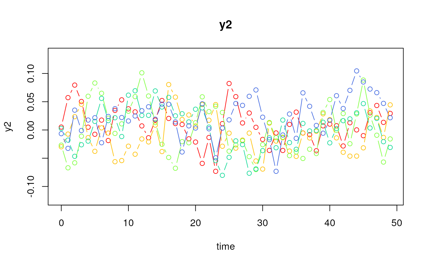
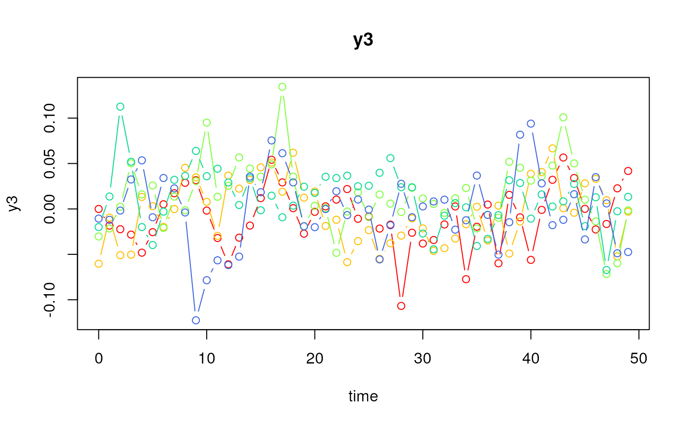
plot(ssm)




# Type 1
ssm <- SimSSMVARFixed(
  n = n,
  time = time,
  mu0 = mu0,
  sigma0_l = sigma0_l,
  alpha = alpha,
  beta = beta,
  psi_l = psi_l,
  type = 1,
  x = x,
  gamma = gamma
)

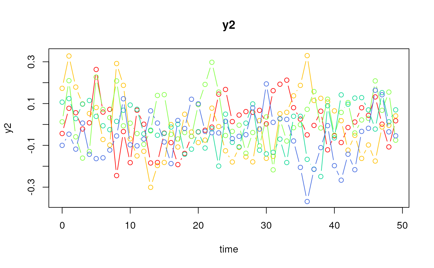
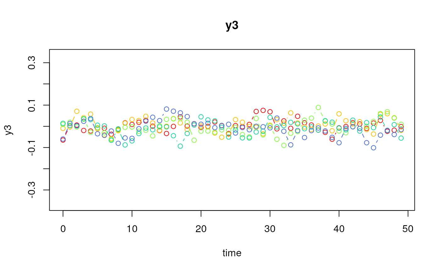
plot(ssm)