Simulate Data from the Linear Growth Curve Model (Individual-Varying Parameters)

This function simulates data from the linear growth curve model. It assumes that the parameters can vary across individuals.

Usage

SimSSMLinGrowthIVary(
  n,
  time,
  mu0,
  sigma0_l,
  theta_l,
  type = 0,
  x = NULL,
  gamma = NULL,
  kappa = NULL
)

Arguments

n: Positive integer. Number of individuals.
time: Positive integer. Number of time points.
mu0: A list of numeric vectors. Each element of the list is a vector of length two. The first element is the mean of the intercept, and the second element is the mean of the slope.
sigma0_l: A list of numeric matrices. Each element of the list is the Cholesky factorization (t(chol(sigma0))) of the covariance matrix of the intercept and the slope.
theta_l: A list numeric values. Each element of the list is the square root of the common measurement error variance.
type: Integer. State space model type. See Details in SimSSMLinGrowth() for more information.
x: List. Each element of the list is a matrix of covariates for each individual i in n. The number of columns in each matrix should be equal to time.
gamma: List of numeric matrices. Each element of the list is the matrix linking the covariates to the latent variables at current time point (\(\boldsymbol{\Gamma}\)).
kappa: List of numeric matrices. Each element of the list is the matrix linking the covariates to the observed variables at current time point (\(\boldsymbol{\kappa}\)).

Value

Returns an object of class simstatespace which is a list with the following elements:

call: Function call.
args: Function arguments.
data: Generated data which is a list of length n. Each element of data is a list with the following elements:
- id: A vector of ID numbers with length l, where l is the value of the function argument time.
- time: A vector time points of length l.
- y: A l by k matrix of values for the manifest variables.
- eta: A l by p matrix of values for the latent variables.
- x: A l by j matrix of values for the covariates (when covariates are included).
fun: Function used.

Details

Parameters can vary across individuals by providing a list of parameter values. If the length of any of the parameters (mu0, sigma0, mu, theta_l, gamma, or kappa) is less the n, the function will cycle through the available values.

References

Chow, S.-M., Ho, M. R., Hamaker, E. L., & Dolan, C. V. (2010). Equivalence and differences between structural equation modeling and state-space modeling techniques. Structural Equation Modeling: A Multidisciplinary Journal, 17(2), 303–332. doi:10.1080/10705511003661553

Author

Ivan Jacob Agaloos Pesigan

Examples

# prepare parameters
# In this example, the mean vector of the intercept and slope vary.
# Specifically,
# there are two sets of values representing two latent classes.
set.seed(42)
## number of individuals
n <- 10
## time points
time <- 5
## dynamic structure
p <- 2
mu0_1 <- c(0.615, 1.006) # lower starting point, higher growth
mu0_2 <- c(1.000, 0.500) # higher starting point, lower growth
mu0 <- list(mu0_1, mu0_2)
sigma0 <- matrix(
  data = c(
    1.932,
    0.618,
    0.618,
    0.587
  ),
  nrow = p
)
sigma0_l <- list(t(chol(sigma0)))
## measurement model
k <- 1
theta <- 0.50
theta_l <- list(sqrt(theta))
## covariates
j <- 2
x <- lapply(
  X = seq_len(n),
  FUN = function(i) {
    matrix(
      data = stats::rnorm(n = time * j),
      nrow = j,
      ncol = time
    )
  }
)
gamma <- list(
  diag(x = 0.10, nrow = p, ncol = j)
)
kappa <- list(
  diag(x = 0.10, nrow = k, ncol = j)
)

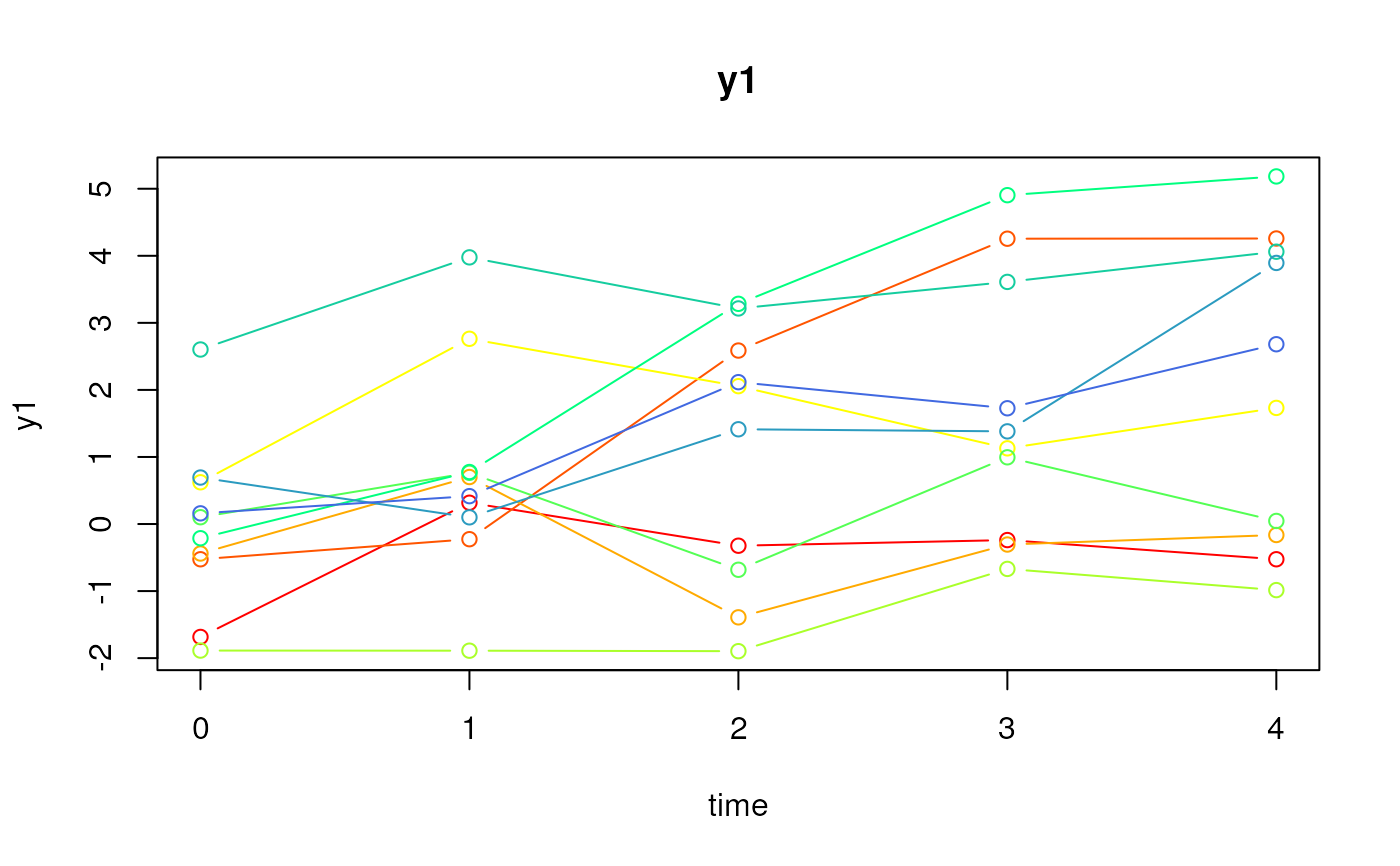
# Type 0
ssm <- SimSSMLinGrowthIVary(
  n = n,
  time = time,
  mu0 = mu0,
  sigma0_l = sigma0_l,
  theta_l = theta_l,
  type = 0
)

plot(ssm)


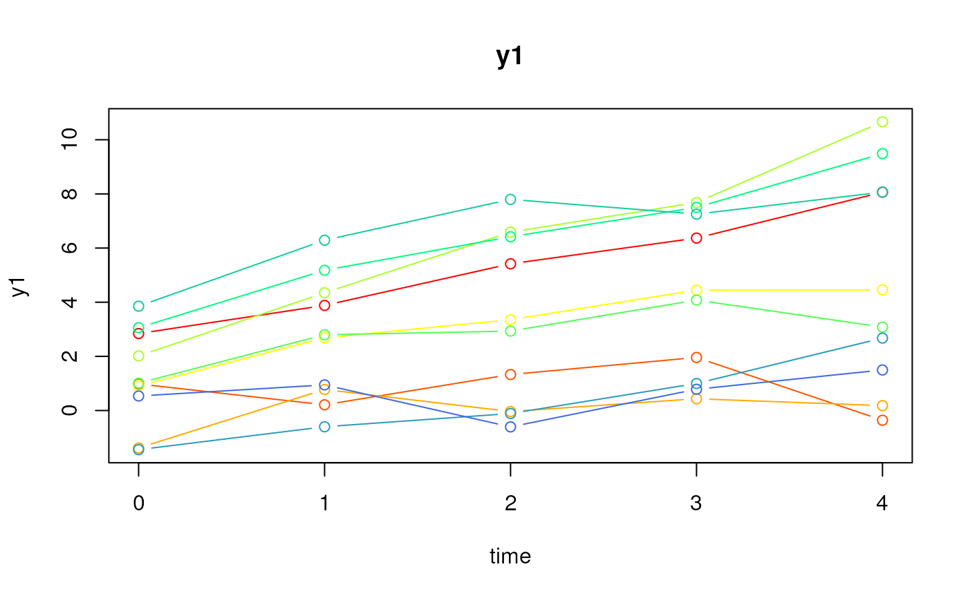# Type 1
ssm <- SimSSMLinGrowthIVary(
  n = n,
  time = time,
  mu0 = mu0,
  sigma0_l = sigma0_l,
  theta_l = theta_l,
  type = 1,
  x = x,
  gamma = gamma
)

plot(ssm)


# Type 2
ssm <- SimSSMLinGrowthIVary(
  n = n,
  time = time,
  mu0 = mu0,
  sigma0_l = sigma0_l,
  theta_l = theta_l,
  type = 2,
  x = x,
  gamma = gamma,
  kappa = kappa
)

plot(ssm)