Simulate Data from the Linear Growth Curve Model
Source:R/simStateSpace-sim-ssm-lin-growth.R
SimSSMLinGrowth.RdThis function simulates data from the linear growth curve model.
Usage
SimSSMLinGrowth(
  n,
  time,
  mu0,
  sigma0_l,
  theta_l,
  type = 0,
  x = NULL,
  gamma = NULL,
  kappa = NULL
)
Arguments
- n
Positive integer. Number of individuals.
- time
Positive integer. Number of time points.
- mu0
Numeric vector. A vector of length two. The first element is the mean of the intercept, and the second element is the mean of the slope.
- sigma0_l
Numeric matrix. Cholesky factorization (
t(chol(sigma0))) of the covariance matrix of the intercept and the slope.- theta_l
Numeric. Square root of the common measurement error variance.
- type
Integer. State space model type. See Details for more information.
- x
List. Each element of the list is a matrix of covariates for each individual
iinn. The number of columns in each matrix should be equal totime.- gamma
Numeric matrix. Matrix linking the covariates to the latent variables at current time point (\(\boldsymbol{\Gamma}\)).
- kappa
Numeric matrix. Matrix linking the covariates to the observed variables at current time point (\(\boldsymbol{\kappa}\)).
Value
Returns an object of class simstatespace
which is a list with the following elements:
call: Function call.args: Function arguments.data: Generated data which is a list of lengthn. Each element ofdatais a list with the following elements:id: A vector of ID numbers with lengthl, wherelis the value of the function argumenttime.time: A vector time points of lengthl.y: Albykmatrix of values for the manifest variables.eta: Albypmatrix of values for the latent variables.x: Albyjmatrix of values for the covariates (when covariates are included).
fun: Function used.
Details
Type 0
The measurement model is given by $$ Y_{i, t} = \left( \begin{array}{cc} 1 & 0 \\ \end{array} \right) \left( \begin{array}{c} \eta_{0_{i, t}} \\ \eta_{1_{i, t}} \\ \end{array} \right) + \boldsymbol{\varepsilon}_{i, t}, \quad \mathrm{with} \quad \boldsymbol{\varepsilon}_{i, t} \sim \mathcal{N} \left( 0, \theta \right) $$ where \(Y_{i, t}\), \(\eta_{0_{i, t}}\), \(\eta_{1_{i, t}}\), and \(\boldsymbol{\varepsilon}_{i, t}\) are random variables and \(\theta\) is a model parameter. \(Y_{i, t}\) is the observed random variable at time \(t\) and individual \(i\), \(\eta_{0_{i, t}}\) (intercept) and \(\eta_{1_{i, t}}\) (slope) form a vector of latent random variables at time \(t\) and individual \(i\), and \(\boldsymbol{\varepsilon}_{i, t}\) a vector of random measurement errors at time \(t\) and individual \(i\). \(\theta\) is the variance of \(\boldsymbol{\varepsilon}\).
The dynamic structure is given by $$ \left( \begin{array}{c} \eta_{0_{i, t}} \\ \eta_{1_{i, t}} \\ \end{array} \right) = \left( \begin{array}{cc} 1 & 1 \\ 0 & 1 \\ \end{array} \right) \left( \begin{array}{c} \eta_{0_{i, t - 1}} \\ \eta_{1_{i, t - 1}} \\ \end{array} \right) . $$
The mean vector and covariance matrix of the intercept and slope are captured in the mean vector and covariance matrix of the initial condition given by $$ \boldsymbol{\mu}_{\boldsymbol{\eta} \mid 0} = \left( \begin{array}{c} \mu_{\eta_{0}} \\ \mu_{\eta_{1}} \\ \end{array} \right) \quad \mathrm{and,} $$
$$ \boldsymbol{\Sigma}_{\boldsymbol{\eta} \mid 0} = \left( \begin{array}{cc} \sigma^{2}_{\eta_{0}} & \sigma_{\eta_{0}, \eta_{1}} \\ \sigma_{\eta_{1}, \eta_{0}} & \sigma^{2}_{\eta_{1}} \\ \end{array} \right) . $$
Type 1
The measurement model is given by $$ Y_{i, t} = \left( \begin{array}{cc} 1 & 0 \\ \end{array} \right) \left( \begin{array}{c} \eta_{0_{i, t}} \\ \eta_{1_{i, t}} \\ \end{array} \right) + \boldsymbol{\varepsilon}_{i, t}, \quad \mathrm{with} \quad \boldsymbol{\varepsilon}_{i, t} \sim \mathcal{N} \left( 0, \theta \right) . $$
The dynamic structure is given by $$ \left( \begin{array}{c} \eta_{0_{i, t}} \\ \eta_{1_{i, t}} \\ \end{array} \right) = \left( \begin{array}{cc} 1 & 1 \\ 0 & 1 \\ \end{array} \right) \left( \begin{array}{c} \eta_{0_{i, t - 1}} \\ \eta_{1_{i, t - 1}} \\ \end{array} \right) + \boldsymbol{\Gamma} \mathbf{x}_{i, t} $$ where \(\mathbf{x}_{i, t}\) represents a vector of covariates at time \(t\) and individual \(i\), and \(\boldsymbol{\Gamma}\) the coefficient matrix linking the covariates to the latent variables.
Type 2
The measurement model is given by $$ Y_{i, t} = \left( \begin{array}{cc} 1 & 0 \\ \end{array} \right) \left( \begin{array}{c} \eta_{0_{i, t}} \\ \eta_{1_{i, t}} \\ \end{array} \right) + \boldsymbol{\kappa} \mathbf{x}_{i, t} + \boldsymbol{\varepsilon}_{i, t}, \quad \mathrm{with} \quad \boldsymbol{\varepsilon}_{i, t} \sim \mathcal{N} \left( 0, \theta \right) $$ where \(\boldsymbol{\kappa}\) represents the coefficient matrix linking the covariates to the observed variables.
The dynamic structure is given by $$ \left( \begin{array}{c} \eta_{0_{i, t}} \\ \eta_{1_{i, t}} \\ \end{array} \right) = \left( \begin{array}{cc} 1 & 1 \\ 0 & 1 \\ \end{array} \right) \left( \begin{array}{c} \eta_{0_{i, t - 1}} \\ \eta_{1_{i, t - 1}} \\ \end{array} \right) + \boldsymbol{\Gamma} \mathbf{x}_{i, t} . $$
References
Chow, S.-M., Ho, M. R., Hamaker, E. L., & Dolan, C. V. (2010). Equivalence and differences between structural equation modeling and state-space modeling techniques. Structural Equation Modeling: A Multidisciplinary Journal, 17(2), 303-332. doi:10.1080/10705511003661553
See also
Other Simulation of State Space Models Data Functions:
LinSDE2SSM(),
LinSDECovEta(),
LinSDECovY(),
LinSDEInterceptEta(),
LinSDEInterceptY(),
LinSDEMeanEta(),
LinSDEMeanY(),
ProjectToHurwitz(),
ProjectToStability(),
SSMCovEta(),
SSMCovY(),
SSMInterceptEta(),
SSMInterceptY(),
SSMMeanEta(),
SSMMeanY(),
SimAlphaN(),
SimBetaN(),
SimBetaN2(),
SimBetaNCovariate(),
SimCovDiagN(),
SimCovN(),
SimIotaN(),
SimMVN(),
SimMuN(),
SimNuN(),
SimPhiN(),
SimPhiN2(),
SimPhiNCovariate(),
SimSSMFixed(),
SimSSMIVary(),
SimSSMLinGrowthIVary(),
SimSSMLinSDEFixed(),
SimSSMLinSDEIVary(),
SimSSMOUFixed(),
SimSSMOUIVary(),
SimSSMVARFixed(),
SimSSMVARIVary(),
SpectralRadius(),
TestPhi(),
TestPhiHurwitz(),
TestStability(),
TestStationarity()
Examples
# prepare parameters
set.seed(42)
## number of individuals
n <- 5
## time points
time <- 5
## dynamic structure
p <- 2
mu0 <- c(0.615, 1.006)
sigma0 <- matrix(
data = c(
1.932,
0.618,
0.618,
0.587
),
nrow = p
)
sigma0_l <- t(chol(sigma0))
## measurement model
k <- 1
theta <- 0.50
theta_l <- sqrt(theta)
## covariates
j <- 2
x <- lapply(
X = seq_len(n),
FUN = function(i) {
matrix(
data = rnorm(n = j * time),
nrow = j
)
}
)
gamma <- diag(x = 0.10, nrow = p, ncol = j)
kappa <- diag(x = 0.10, nrow = k, ncol = j)
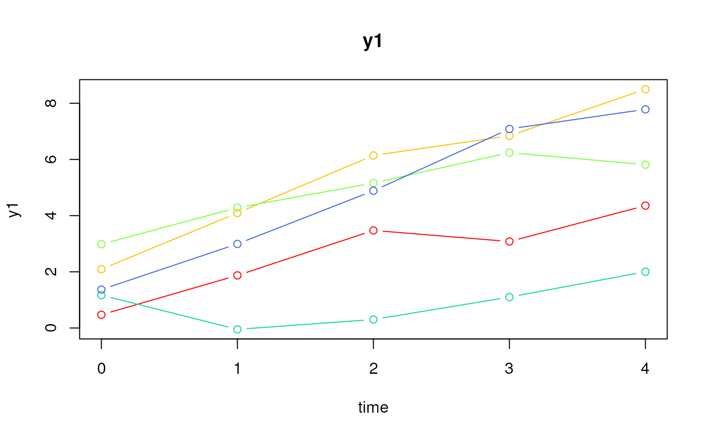
# Type 0
ssm <- SimSSMLinGrowth(
n = n,
time = time,
mu0 = mu0,
sigma0_l = sigma0_l,
theta_l = theta_l,
type = 0
)
plot(ssm)
 # Type 1
ssm <- SimSSMLinGrowth(
n = n,
time = time,
mu0 = mu0,
sigma0_l = sigma0_l,
theta_l = theta_l,
type = 1,
x = x,
gamma = gamma
)
plot(ssm)
# Type 1
ssm <- SimSSMLinGrowth(
n = n,
time = time,
mu0 = mu0,
sigma0_l = sigma0_l,
theta_l = theta_l,
type = 1,
x = x,
gamma = gamma
)
plot(ssm)
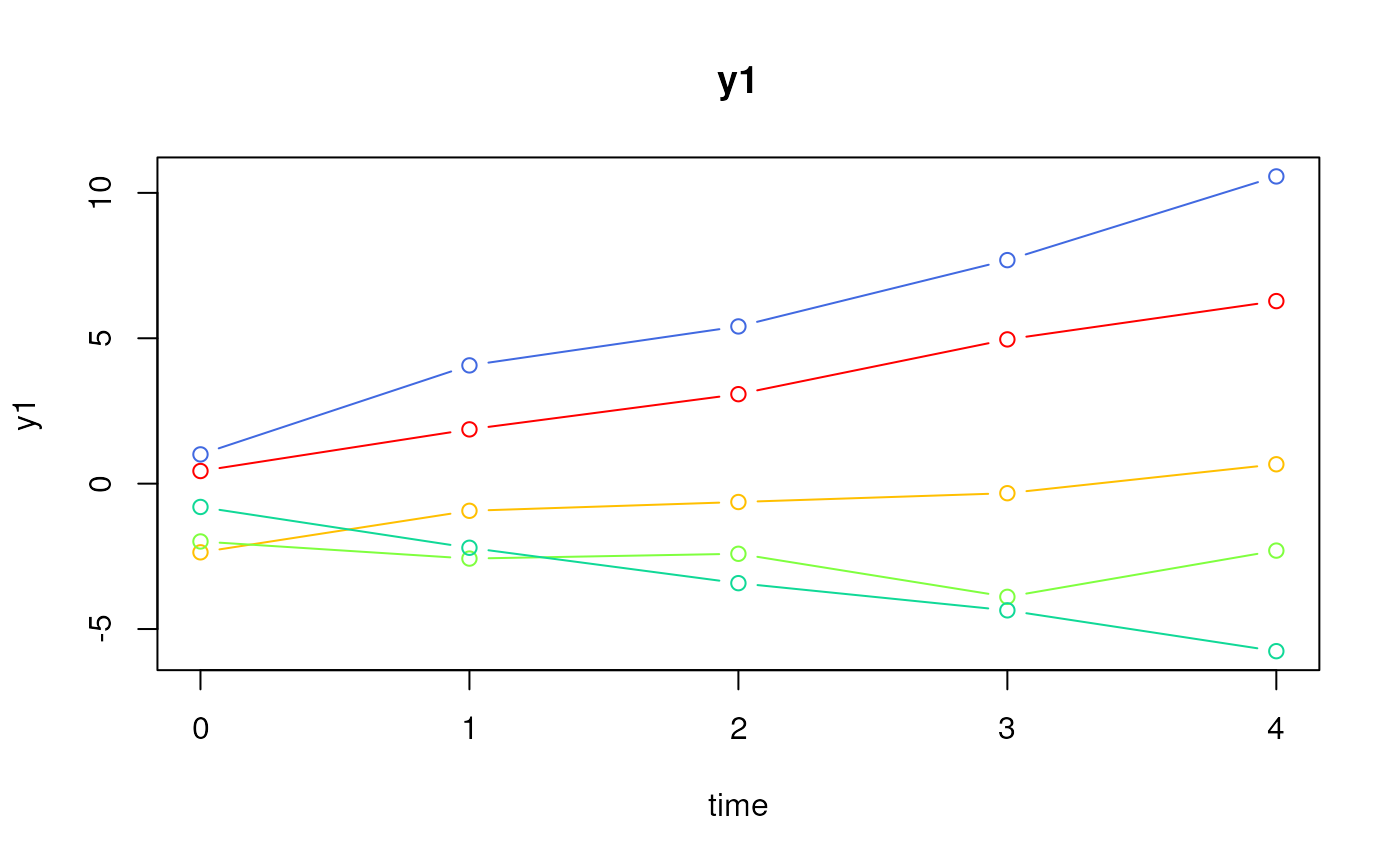 # Type 2
ssm <- SimSSMLinGrowth(
n = n,
time = time,
mu0 = mu0,
sigma0_l = sigma0_l,
theta_l = theta_l,
type = 2,
x = x,
gamma = gamma,
kappa = kappa
)
plot(ssm)
# Type 2
ssm <- SimSSMLinGrowth(
n = n,
time = time,
mu0 = mu0,
sigma0_l = sigma0_l,
theta_l = theta_l,
type = 2,
x = x,
gamma = gamma,
kappa = kappa
)
plot(ssm)
