Simulate Data from the Linear Stochastic Differential Equation Model using a State Space Model Parameterization (Individual-Varying Parameters)

This function simulates data from the linear stochastic differential equation model using a state space model parameterization. It assumes that the parameters can vary across individuals.

Usage

SimSSMLinSDEIVary(
  n,
  time,
  delta_t = 1,
  mu0,
  sigma0_l,
  iota,
  phi,
  sigma_l,
  nu,
  lambda,
  theta_l,
  type = 0,
  x = NULL,
  gamma = NULL,
  kappa = NULL
)

Arguments

n: Positive integer. Number of individuals.
time: Positive integer. Number of time points.
delta_t: Numeric. Time interval. The default value is 1.0 with an option to use a numeric value for the discretized state space model parameterization of the linear stochastic differential equation model.
mu0: List of numeric vectors. Each element of the list is the mean of initial latent variable values (\(\boldsymbol{\mu}_{\boldsymbol{\eta} \mid 0}\)).
sigma0_l: List of numeric matrices. Each element of the list is the Cholesky factorization (t(chol(sigma0))) of the covariance matrix of initial latent variable values (\(\boldsymbol{\Sigma}_{\boldsymbol{\eta} \mid 0}\)).
iota: List of numeric vectors. Each element of the list is an unobserved term that is constant over time (\(\boldsymbol{\iota}\)).
phi: List of numeric matrix. Each element of the list is the drift matrix which represents the rate of change of the solution in the absence of any random fluctuations (\(\boldsymbol{\Phi}\)).
sigma_l: List of numeric matrix. Each element of the list is the Cholesky factorization (t(chol(sigma))) of the covariance matrix of volatility or randomness in the process \(\boldsymbol{\Sigma}\).
nu: List of numeric vectors. Each element of the list is the vector of intercept values for the measurement model (\(\boldsymbol{\nu}\)).
lambda: List of numeric matrices. Each element of the list is the factor loading matrix linking the latent variables to the observed variables (\(\boldsymbol{\Lambda}\)).
theta_l: List of numeric matrices. Each element of the list is the Cholesky factorization (t(chol(theta))) of the covariance matrix of the measurement error (\(\boldsymbol{\Theta}\)).
type: Integer. State space model type. See Details in SimSSMLinSDEFixed() for more information.
x: List. Each element of the list is a matrix of covariates for each individual i in n. The number of columns in each matrix should be equal to time.
gamma: List of numeric matrices. Each element of the list is the matrix linking the covariates to the latent variables at current time point (\(\boldsymbol{\Gamma}\)).
kappa: List of numeric matrices. Each element of the list is the matrix linking the covariates to the observed variables at current time point (\(\boldsymbol{\kappa}\)).

Value

Returns an object of class simstatespace which is a list with the following elements:

call: Function call.
args: Function arguments.
data: Generated data which is a list of length n. Each element of data is a list with the following elements:
- id: A vector of ID numbers with length l, where l is the value of the function argument time.
- time: A vector time points of length l.
- y: A l by k matrix of values for the manifest variables.
- eta: A l by p matrix of values for the latent variables.
- x: A l by j matrix of values for the covariates (when covariates are included).
fun: Function used.

Details

Parameters can vary across individuals by providing a list of parameter values. If the length of any of the parameters (mu0, sigma0_l, iota, phi, sigma_l, nu, lambda, theta_l, gamma, or kappa) is less the n, the function will cycle through the available values.

References

Chow, S.-M., Ho, M. R., Hamaker, E. L., & Dolan, C. V. (2010). Equivalence and differences between structural equation modeling and state-space modeling techniques. Structural Equation Modeling: A Multidisciplinary Journal, 17(2), 303–332. doi:10.1080/10705511003661553

Chow, S.-M., Losardo, D., Park, J., & Molenaar, P. C. M. (2023). Continuous-time dynamic models: Connections to structural equation models and other discrete-time models. In R. H. Hoyle (Ed.), Handbook of structural equation modeling (2nd ed.). The Guilford Press.

Harvey, A. C. (1990). Forecasting, structural time series models and the Kalman filter. Cambridge University Press. doi:10.1017/cbo9781107049994

Author

Ivan Jacob Agaloos Pesigan

Examples

# prepare parameters
# In this example, phi varies across individuals.
set.seed(42)
## number of individuals
n <- 5
## time points
time <- 50
delta_t <- 0.10
## dynamic structure
p <- 2
mu0 <- list(
  c(-3.0, 1.5)
)
sigma0 <- 0.001 * diag(p)
sigma0_l <- list(
  t(chol(sigma0))
)
iota <- list(
  c(0.317, 0.230)
)
phi <- list(
  -0.1 * diag(p),
  -0.2 * diag(p),
  -0.3 * diag(p),
  -0.4 * diag(p),
  -0.5 * diag(p)
)
sigma <- matrix(
  data = c(
    2.79,
    0.06,
    0.06,
    3.27
  ),
  nrow = p
)
sigma_l <- list(
  t(chol(sigma))
)
## measurement model
k <- 2
nu <- list(
  rep(x = 0, times = k)
)
lambda <- list(
  diag(k)
)
theta <- 0.001 * diag(k)
theta_l <- list(
  t(chol(theta))
)
## covariates
j <- 2
x <- lapply(
  X = seq_len(n),
  FUN = function(i) {
    matrix(
      data = stats::rnorm(n = time * j),
      nrow = j,
      ncol = time
    )
  }
)
gamma <- list(
  diag(x = 0.10, nrow = p, ncol = j)
)
kappa <- list(
  diag(x = 0.10, nrow = k, ncol = j)
)

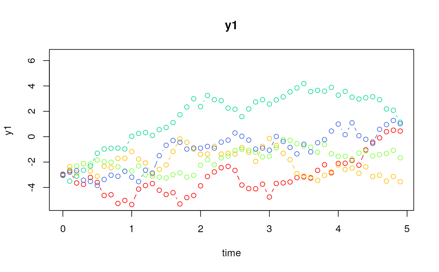
# Type 0
ssm <- SimSSMLinSDEIVary(
  n = n,
  time = time,
  delta_t = delta_t,
  mu0 = mu0,
  sigma0_l = sigma0_l,
  iota = iota,
  phi = phi,
  sigma_l = sigma_l,
  nu = nu,
  lambda = lambda,
  theta_l = theta_l,
  type = 0
)

plot(ssm)



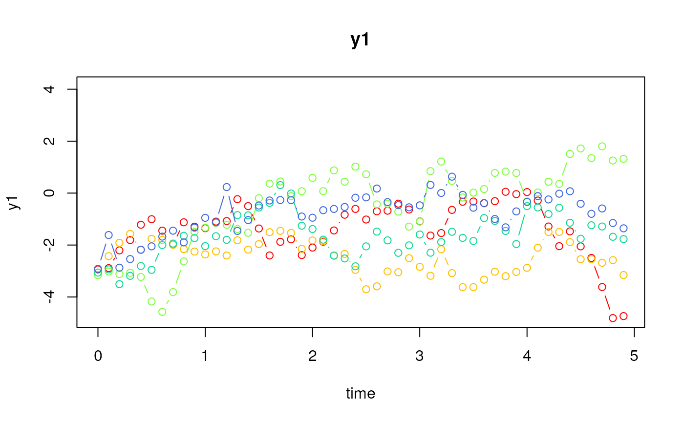
# Type 1
ssm <- SimSSMLinSDEIVary(
  n = n,
  time = time,
  delta_t = delta_t,
  mu0 = mu0,
  sigma0_l = sigma0_l,
  iota = iota,
  phi = phi,
  sigma_l = sigma_l,
  nu = nu,
  lambda = lambda,
  theta_l = theta_l,
  type = 1,
  x = x,
  gamma = gamma
)

plot(ssm)



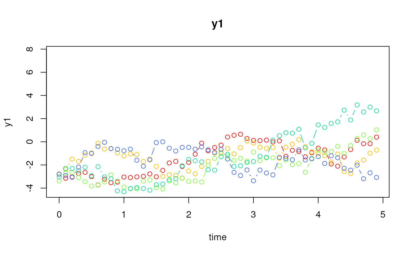
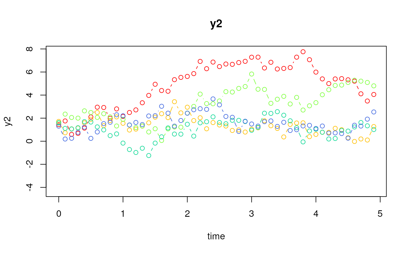
# Type 2
ssm <- SimSSMLinSDEIVary(
  n = n,
  time = time,
  delta_t = delta_t,
  mu0 = mu0,
  sigma0_l = sigma0_l,
  iota = iota,
  phi = phi,
  sigma_l = sigma_l,
  nu = nu,
  lambda = lambda,
  theta_l = theta_l,
  type = 2,
  x = x,
  gamma = gamma,
  kappa = kappa
)

plot(ssm)