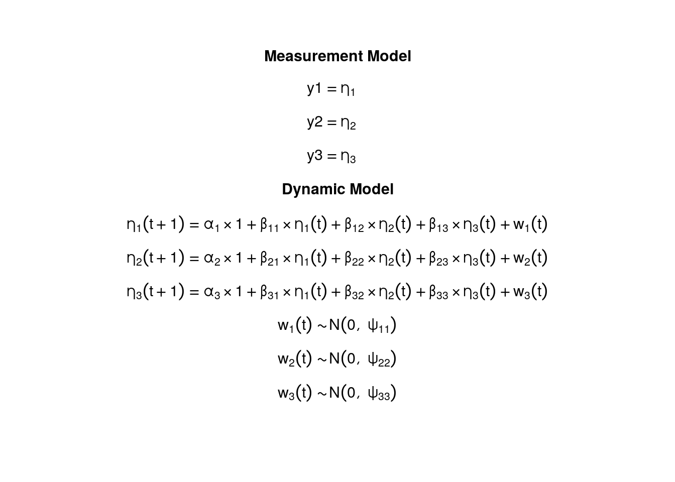
Model
The measurement model is given by \[\begin{equation}
\mathbf{y}_{i, t}
=
\boldsymbol{\eta}_{i, t}
\end{equation}\] where \(\mathbf{y}_{i, t}\) represents a vector of observed variables and \(\boldsymbol{\eta}_{i, t}\) a vector of latent variables for individual \(i\) and time \(t\) . Since the observed and latent variables are equal, we only generate data from the dynamic structure.
The dynamic structure is given by \[\begin{equation}
\boldsymbol{\eta}_{i, t}
=
\boldsymbol{\alpha}
+
\boldsymbol{\beta}
\boldsymbol{\eta}_{i, t - 1}
+
\boldsymbol{\zeta}_{i, t},
\quad
\mathrm{with}
\quad
\boldsymbol{\zeta}_{i, t}
\sim
\mathcal{N}
\left(
\mathbf{0},
\boldsymbol{\Psi}
\right)
\end{equation}\] where \(\boldsymbol{\eta}_{i, t}\) , \(\boldsymbol{\eta}_{i, t - 1}\) , and \(\boldsymbol{\zeta}_{i, t}\) are random variables, and \(\boldsymbol{\alpha}\) , \(\boldsymbol{\beta}\) , and \(\boldsymbol{\Psi}\) are model parameters. Here, \(\boldsymbol{\eta}_{i, t}\) is a vector of latent variables at time \(t\) and individual \(i\) , \(\boldsymbol{\eta}_{i, t - 1}\) represents a vector of latent variables at time \(t - 1\) and individual \(i\) , and \(\boldsymbol{\zeta}_{i, t}\) represents a vector of dynamic noise at time \(t\) and individual \(i\) . \(\boldsymbol{\alpha}\) denotes a vector of intercepts, \(\boldsymbol{\beta}\) a matrix of autoregression and cross regression coefficients, and \(\boldsymbol{\Psi}\) the covariance matrix of \(\boldsymbol{\zeta}_{i, t}\) .
An alternative representation of the dynamic noise is given by \[\begin{equation}
\boldsymbol{\zeta}_{i, t}
=
\boldsymbol{\Psi}^{\frac{1}{2}}
\mathbf{z}_{i, t},
\quad
\mathrm{with}
\quad
\mathbf{z}_{i, t}
\sim
\mathcal{N}
\left(
\mathbf{0},
\mathbf{I}
\right)
\end{equation}\] where \(\left( \boldsymbol{\Psi}^{\frac{1}{2}} \right) \left( \boldsymbol{\Psi}^{\frac{1}{2}} \right)^{\prime} = \boldsymbol{\Psi}\) .
Data Generation
Notation
Let \(t = 1000\) be the number of time points and \(n = 5\) be the number of individuals.
Let the initial condition \(\boldsymbol{\eta}_{0}\) be given by
\[\begin{equation}
\boldsymbol{\eta}_{0} \sim \mathcal{N} \left( \boldsymbol{\mu}_{\boldsymbol{\eta} \mid 0}, \boldsymbol{\Sigma}_{\boldsymbol{\eta} \mid 0} \right)
\end{equation}\]
\[\begin{equation}
\boldsymbol{\mu}_{\boldsymbol{\eta} \mid 0}
=
\left(
\begin{array}{c}
0 \\
0 \\
0 \\
\end{array}
\right)
\end{equation}\]
\[\begin{equation}
\boldsymbol{\Sigma}_{\boldsymbol{\eta} \mid 0}
=
\left(
\begin{array}{ccc}
1 & 0.2 & 0.2 \\
0.2 & 1 & 0.2 \\
0.2 & 0.2 & 1 \\
\end{array}
\right) .
\end{equation}\]
Let the constant vector \(\boldsymbol{\alpha}\) be given by
\[\begin{equation}
\boldsymbol{\alpha}
=
\left(
\begin{array}{c}
0 \\
0 \\
0 \\
\end{array}
\right) .
\end{equation}\]
Let the transition matrix \(\boldsymbol{\beta}\) be given by
\[\begin{equation}
\boldsymbol{\beta}
=
\left(
\begin{array}{ccc}
0.7 & 0 & 0 \\
0.5 & 0.6 & 0 \\
-0.1 & 0.4 & 0.5 \\
\end{array}
\right) .
\end{equation}\]
Let the dynamic process noise \(\boldsymbol{\Psi}\) be given by
\[\begin{equation}
\boldsymbol{\Psi}
=
\left(
\begin{array}{ccc}
0.1 & 0 & 0 \\
0 & 0.1 & 0 \\
0 & 0 & 0.1 \\
\end{array}
\right) .
\end{equation}\]
R Function Arguments
     [,1] [,2] [,3]
[1,]  1.0  0.2  0.2
[2,]  0.2  1.0  0.2
[3,]  0.2  0.2  1.0
sigma0_l # sigma0_l <- t(chol(sigma0))
     [,1]      [,2]      [,3]
[1,]  1.0 0.0000000 0.0000000
[2,]  0.2 0.9797959 0.0000000
[3,]  0.2 0.1632993 0.9660918
     [,1] [,2] [,3]
[1,]  0.7  0.0  0.0
[2,]  0.5  0.6  0.0
[3,] -0.1  0.4  0.5
     [,1] [,2] [,3]
[1,]  0.1  0.0  0.0
[2,]  0.0  0.1  0.0
[3,]  0.0  0.0  0.1
psi_l # psi_l <- t(chol(psi))
          [,1]      [,2]      [,3]
[1,] 0.3162278 0.0000000 0.0000000
[2,] 0.0000000 0.3162278 0.0000000
[3,] 0.0000000 0.0000000 0.3162278
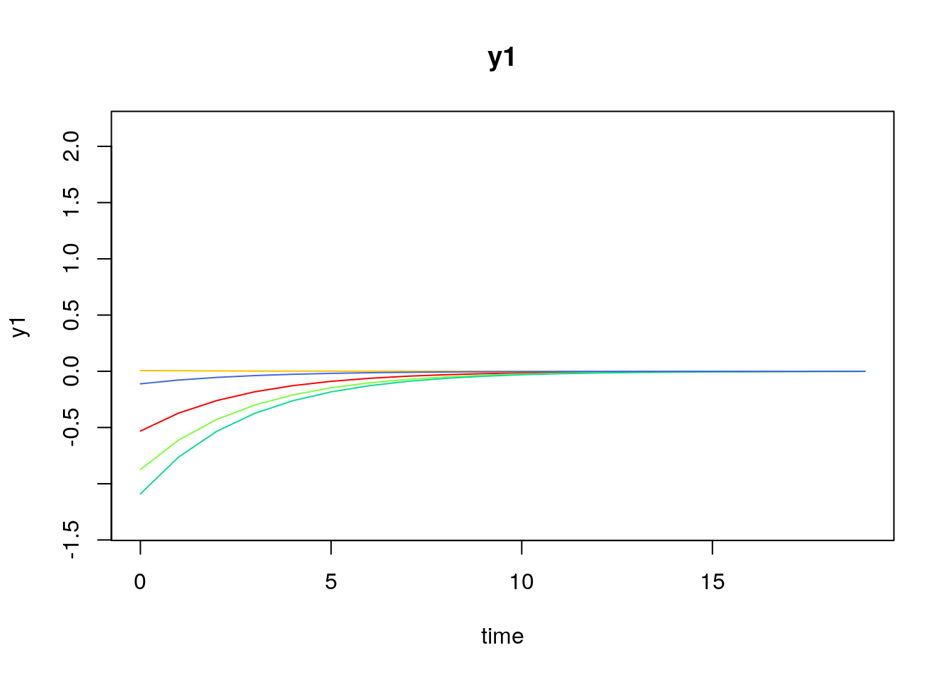
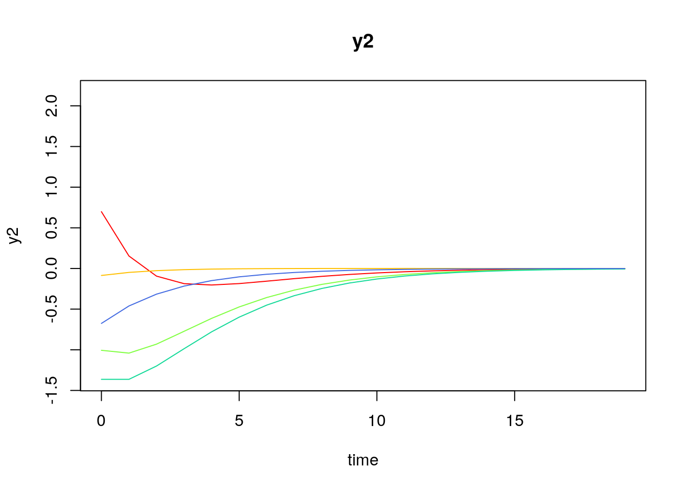
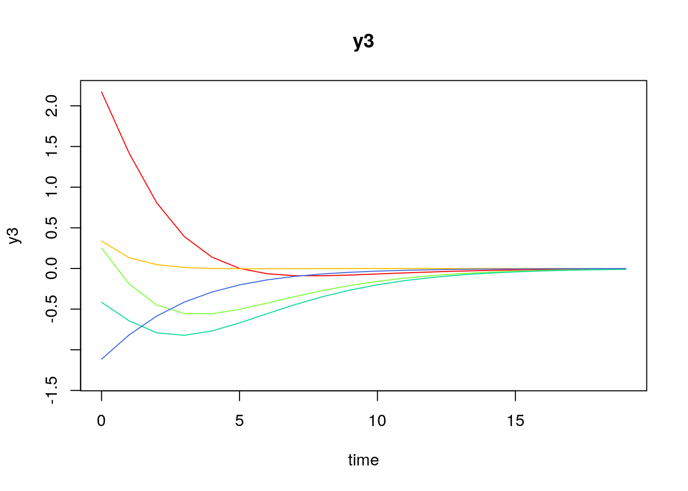
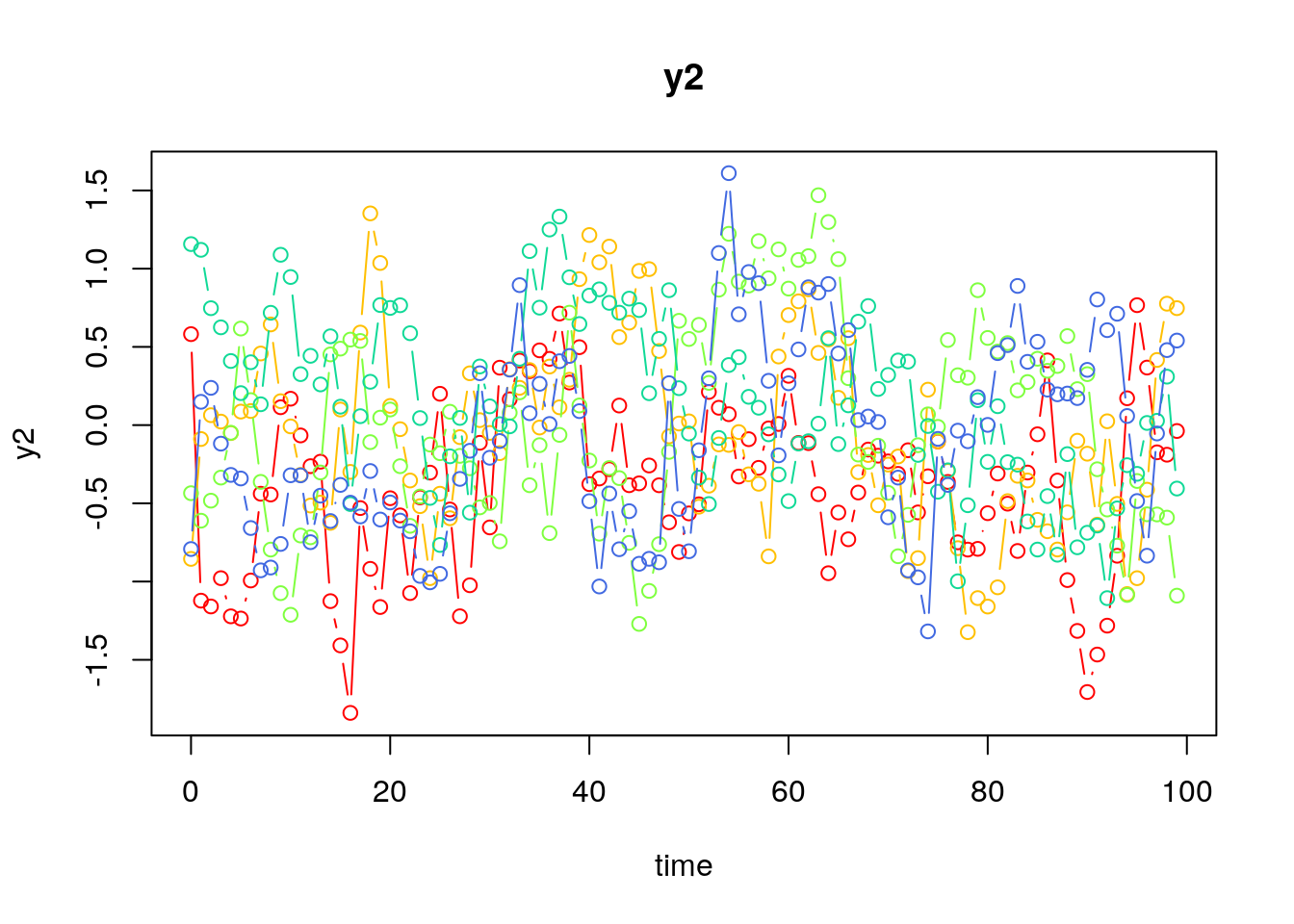
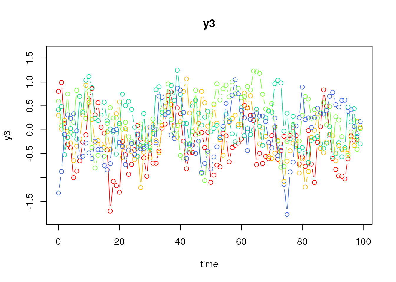
Visualizing the Dynamics Without Process Noise (n = 5 with Different Initial Condition)
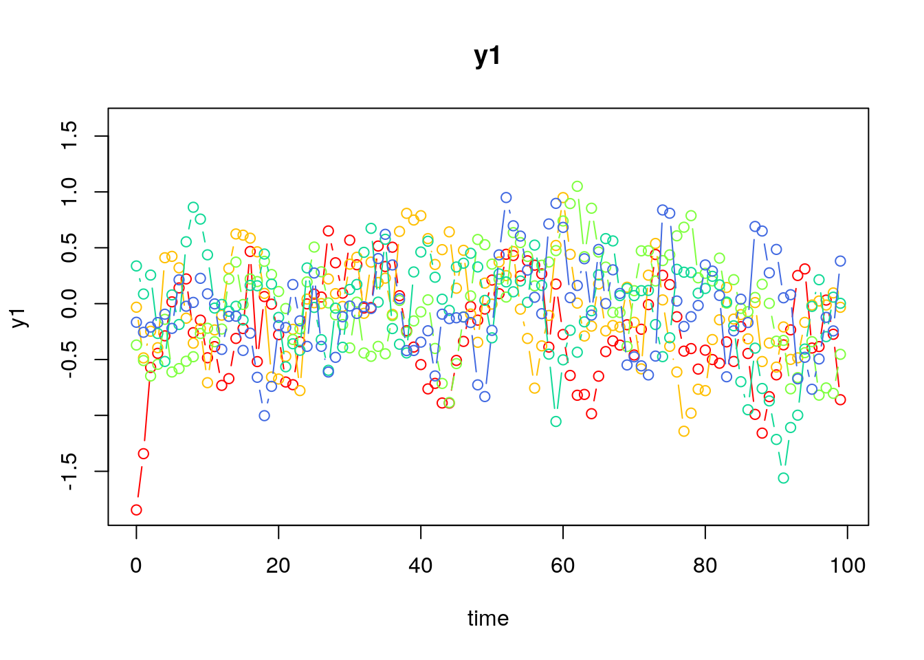
Using the SimSSMVARFixed Function from the simStateSpace Package to Simulate Data
  id time          y1         y2         y3
1  1    0 -1.84569501  0.5815402  0.8057225
2  1    1 -1.34252674 -1.1219724  0.9873906
3  1    2 -0.57123433 -1.1591679  0.1280274
4  1    3 -0.44448720 -0.9783200 -0.3028425
5  1    4 -0.28796224 -1.2222325 -0.3807219
6  1    5  0.01622801 -1.2362032 -1.0056038
       id         time             y1                 y2
 Min.   :1   Min.   :  0.0   Min.   :-1.84570   Min.   :-2.17817
 1st Qu.:2   1st Qu.:249.8   1st Qu.:-0.31071   1st Qu.:-0.42138
 Median :3   Median :499.5   Median :-0.01764   Median :-0.01740
 Mean   :3   Mean   :499.5   Mean   :-0.01425   Mean   :-0.02021
 3rd Qu.:4   3rd Qu.:749.2   3rd Qu.: 0.27870   3rd Qu.: 0.37021
 Max.   :5   Max.   :999.0   Max.   : 1.56537   Max.   : 2.83572
       y3
 Min.   :-1.774215
 1st Qu.:-0.363420
 Median :-0.005834
 Mean   :-0.009098
 3rd Qu.: 0.341318
 Max.   : 1.817859
Model Fitting
Prepare Data
dynr_data <- dynr :: dynr.data ( data = data ,
id = "id" ,
time = "time" ,
observed = c ( "y1" , "y2" , "y3" )
)
Prepare Initial Condition
dynr_initial <- dynr :: prep.initial ( values.inistate = mu0 ,
params.inistate = c ( "mu0_1_1" , "mu0_2_1" , "mu0_3_1" ) ,
values.inicov = sigma0 ,
params.inicov = matrix (
data = c (
"sigma0_1_1" , "sigma0_2_1" , "sigma0_3_1" ,
"sigma0_2_1" , "sigma0_2_2" , "sigma0_3_2" ,
"sigma0_3_1" , "sigma0_3_2" , "sigma0_3_3"
) ,
nrow = 3
)
)
Prepare Measurement Model
dynr_measurement <- dynr :: prep.measurement ( values.load = diag ( 3 ) ,
params.load = matrix ( data = "fixed" , nrow = 3 , ncol = 3 ) ,
state.names = c ( "eta_1" , "eta_2" , "eta_3" ) ,
obs.names = c ( "y1" , "y2" , "y3" )
)
Prepare Dynamic Process
dynr_dynamics <- dynr :: prep.formulaDynamics ( formula = list (
eta_1 ~ alpha_1_1 * 1 + beta_1_1 * eta_1 + beta_1_2 * eta_2 + beta_1_3 * eta_3 ,
eta_2 ~ alpha_2_1 * 1 + beta_2_1 * eta_1 + beta_2_2 * eta_2 + beta_2_3 * eta_3 ,
eta_3 ~ alpha_3_1 * 1 + beta_3_1 * eta_1 + beta_3_2 * eta_2 + beta_3_3 * eta_3
) ,
startval = c (
alpha_1_1 = alpha [ 1 ] , alpha_2_1 = alpha [ 2 ] , alpha_3_1 = alpha [ 3 ] ,
beta_1_1 = beta [ 1 , 1 ] , beta_1_2 = beta [ 1 , 2 ] , beta_1_3 = beta [ 1 , 3 ] ,
beta_2_1 = beta [ 2 , 1 ] , beta_2_2 = beta [ 2 , 2 ] , beta_2_3 = beta [ 2 , 3 ] ,
beta_3_1 = beta [ 3 , 1 ] , beta_3_2 = beta [ 3 , 2 ] , beta_3_3 = beta [ 3 , 3 ]
) ,
isContinuousTime = FALSE
)
Prepare Process Noise
dynr_noise <- dynr :: prep.noise ( values.latent = psi ,
params.latent = matrix (
data = c (
"psi_1_1" , "psi_2_1" , "psi_3_1" ,
"psi_2_1" , "psi_2_2" , "psi_3_2" ,
"psi_3_1" , "psi_3_2" , "psi_3_3"
) ,
nrow = 3
) ,
values.observed = matrix ( data = 0 , nrow = 3 , ncol = 3 ) ,
params.observed = matrix ( data = "fixed" , nrow = 3 , ncol = 3 )
)
Prepare the Model
model <- dynr :: dynr.model ( data = dynr_data ,
initial = dynr_initial ,
measurement = dynr_measurement ,
dynamics = dynr_dynamics ,
noise = dynr_noise ,
outfile = "var.c"
)
Fit the Model
results <- dynr :: dynr.cook ( model ,
debug_flag = TRUE ,
verbose = FALSE
)
[1] "Get ready!!!!"
using C compiler: ‘gcc (Ubuntu 13.3.0-6ubuntu2~24.04) 13.3.0’
Optimization function called.
Starting Hessian calculation ...
Finished Hessian calculation.
Original exit flag:  3
Modified exit flag:  3
Optimization terminated successfully: ftol_rel or ftol_abs was reached.
Original fitted parameters:  -0.003531293 -0.001280376 0.001523566 0.6895684
0.01390681 -0.003940273 0.4892806 0.6166874 -0.00850994 -0.1131785 0.4157686
0.4948645 -2.314722 -0.02295081 -0.01630225 -2.301541 -0.01437825 -2.302993
-0.7217189 0.5433516 0.8634073 -0.2858639 -1.244706 0.1022364 0.00547225
0.08818863 -1.187881

Transformed fitted parameters:  -0.003531293 -0.001280376 0.001523566 0.6895684
0.01390681 -0.003940273 0.4892806 0.6166874 -0.00850994 -0.1131785 0.4157686
0.4948645 0.09879361 -0.002267393 -0.001610558 0.1001565 -0.001402363 0.1000062
-0.7217189 0.5433516 0.8634073 0.7513649 -0.9352283 0.07681685 2.169571
-0.006941846 0.3205399

Doing end processing
Successful trial
Total Time: 2.207808
Backend Time: 2.200906
Summary
Coefficients:
             Estimate Std. Error t value   ci.lower   ci.upper Pr(>|t|)
alpha_1_1  -0.0035313  0.0044508  -0.793 -0.0122548  0.0051922   0.2138
alpha_2_1  -0.0012804  0.0044814  -0.286 -0.0100638  0.0075031   0.3876
alpha_3_1   0.0015236  0.0044781   0.340 -0.0072533  0.0103004   0.3668
beta_1_1    0.6895684  0.0112672  61.202  0.6674852  0.7116517   <2e-16 ***
beta_1_2    0.0139068  0.0093820   1.482 -0.0044815  0.0322952   0.0692 .
beta_1_3   -0.0039403  0.0095679  -0.412 -0.0226930  0.0148125   0.3402
beta_2_1    0.4892806  0.0113446  43.129  0.4670456  0.5115157   <2e-16 ***
beta_2_2    0.6166874  0.0094464  65.283  0.5981727  0.6352020   <2e-16 ***
beta_2_3   -0.0085099  0.0096336  -0.883 -0.0273915  0.0103716   0.1885
beta_3_1   -0.1131785  0.0113361  -9.984 -0.1353969 -0.0909601   <2e-16 ***
beta_3_2    0.4157686  0.0094393  44.047  0.3972680  0.4342693   <2e-16 ***
beta_3_3    0.4948645  0.0096263  51.408  0.4759973  0.5137317   <2e-16 ***
psi_1_1     0.0987936  0.0019768  49.976  0.0949191  0.1026681   <2e-16 ***
psi_2_1    -0.0022674  0.0014078  -1.611 -0.0050266  0.0004919   0.0537 .
psi_3_1    -0.0016106  0.0014066  -1.145 -0.0043674  0.0011463   0.1261
psi_2_2     0.1001565  0.0020041  49.975  0.0962285  0.1040845   <2e-16 ***
psi_3_2    -0.0014024  0.0014162  -0.990 -0.0041780  0.0013733   0.1611
psi_3_3     0.1000062  0.0020011  49.976  0.0960841  0.1039282   <2e-16 ***
mu0_1_1    -0.7217189  0.3854554  -1.872 -1.4771977  0.0337599   0.0306 *
mu0_2_1     0.5433516  0.6542311   0.831 -0.7389178  1.8256210   0.2031
mu0_3_1     0.8634073  0.2531618   3.410  0.3672192  1.3595954   0.0003 ***
sigma0_1_1  0.7513649  0.4740246   1.585 -0.1777063  1.6804360   0.0565 .
sigma0_2_1 -0.9352283  0.7049527  -1.327 -2.3169103  0.4464537   0.0923 .
sigma0_3_1  0.0768168  0.2221450   0.346 -0.3585794  0.5122131   0.3648
sigma0_2_2  2.1695715  1.3671181   1.587 -0.5099307  4.8490737   0.0563 .
sigma0_3_2 -0.0069418  0.3726743  -0.019 -0.7373700  0.7234863   0.4926
sigma0_3_3  0.3205399  0.2023250   1.584 -0.0760099  0.7170897   0.0566 .
---
Signif. codes:  0 '***' 0.001 '**' 0.01 '*' 0.05 '.' 0.1 ' ' 1

-2 log-likelihood value at convergence = 8000.08
AIC = 8054.08
BIC = 8230.05
Parameter Estimates
[1] -0.003531293 -0.001280376 0.001523566
           [,1]       [,2]         [,3]
[1,]  0.6895684 0.01390681 -0.003940273
[2,]  0.4892806 0.61668735 -0.008509940
[3,] -0.1131785 0.41576863  0.494864534
             [,1]         [,2]         [,3]
[1,]  0.098793608 -0.002267393 -0.001610558
[2,] -0.002267393  0.100156481 -0.001402363
[3,] -0.001610558 -0.001402363  0.100006157
[1] -0.7217189 0.5433516 0.8634073
            [,1]         [,2]         [,3]
[1,]  0.75136488 -0.935228319  0.076816849
[2,] -0.93522832  2.169571479 -0.006941846
[3,]  0.07681685 -0.006941846  0.320539871