The Ornstein–Uhlenbeck Model

Author

Ivan Jacob Agaloos Pesigan

Model

The measurement model is given by \[\begin{equation} \mathbf{y}_{i, t} = \boldsymbol{\nu} + \boldsymbol{\Lambda} \boldsymbol{\eta}_{i, t} + \boldsymbol{\varepsilon}_{i, t}, \quad \mathrm{with} \quad \boldsymbol{\varepsilon}_{i, t} \sim \mathcal{N} \left( \mathbf{0}, \boldsymbol{\Theta} \right) 
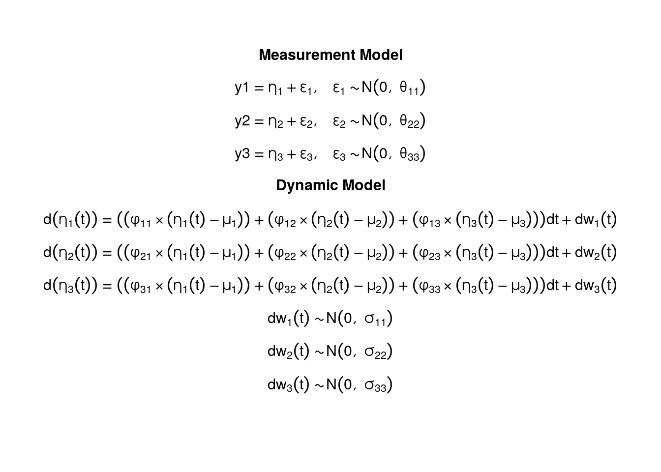
\end{equation}\] where \(\mathbf{y}_{i, t}\), \(\boldsymbol{\eta}_{i, t}\), and \(\boldsymbol{\varepsilon}_{i, t}\) are random variables and \(\boldsymbol{\nu}\), \(\boldsymbol{\Lambda}\), and \(\boldsymbol{\Theta}\) are model parameters. \(\mathbf{y}_{i, t}\) represents a vector of observed random variables, \(\boldsymbol{\eta}_{i, t}\) a vector of latent random variables, and \(\boldsymbol{\varepsilon}_{i, t}\) a vector of random measurement errors, at time \(t\) and individual \(i\). \(\boldsymbol{\nu}\) denotes a vector of intercepts, \(\boldsymbol{\Lambda}\) a matrix of factor loadings, and \(\boldsymbol{\Theta}\) the covariance matrix of \(\boldsymbol{\varepsilon}\).

An alternative representation of the measurement error is given by \[\begin{equation} \boldsymbol{\varepsilon}_{i, t} = \boldsymbol{\Theta}^{\frac{1}{2}} \mathbf{z}_{i, t}, \quad \mathrm{with} \quad \mathbf{z}_{i, t} \sim \mathcal{N} \left( \mathbf{0}, \mathbf{I} \right) \end{equation}\] where \(\mathbf{z}_{i, t}\) is a vector of independent standard normal random variables and \(\left( \boldsymbol{\Theta}^{\frac{1}{2}} \right) \left( \boldsymbol{\Theta}^{\frac{1}{2}} \right)^{\prime} = \boldsymbol{\Theta}\) .

The dynamic structure is given by \[\begin{equation} \mathrm{d} \boldsymbol{\eta}_{i, t} = \boldsymbol{\Phi} \left( \boldsymbol{\eta}_{i, t} - \boldsymbol{\mu} \right) \mathrm{d}t + \boldsymbol{\Sigma}^{\frac{1}{2}} \mathrm{d} \mathbf{W}_{i, t} \end{equation}\] where \(\boldsymbol{\mu}\) is the long-term mean or equilibrium level, \(\boldsymbol{\Phi}\) is the rate of mean reversion, determining how quickly the variable returns to its mean, \(\boldsymbol{\Sigma}\) is the matrix of volatility or randomness in the process, and \(\mathrm{d}\boldsymbol{W}\) is a Wiener process or Brownian motion, which represents random fluctuations.

Data Generation

Notation

Let \(t = 1000\) be the number of time points and \(n = 5\) be the number of individuals.

Let the measurement model intecept vector \(\boldsymbol{\nu}\) be given by

\[\begin{equation} \boldsymbol{\nu} = \left( \begin{array}{c} 0 \\ 0 \\ 0 \\ \end{array} \right) . \end{equation}\]

Let the factor loadings matrix \(\boldsymbol{\Lambda}\) be given by

\[\begin{equation} \boldsymbol{\Lambda} = \left( \begin{array}{ccc} 1 & 0 & 0 \\ 0 & 1 & 0 \\ 0 & 0 & 1 \\ \end{array} \right) . \end{equation}\]

Let the measurement error covariance matrix \(\boldsymbol{\Theta}\) be given by

\[\begin{equation} \boldsymbol{\Theta} = \left( \begin{array}{ccc} 0.2 & 0 & 0 \\ 0 & 0.2 & 0 \\ 0 & 0 & 0.2 \\ \end{array} \right) . \end{equation}\]

Let the initial condition \(\boldsymbol{\eta}_{0}\) be given by

\[\begin{equation} \boldsymbol{\eta}_{0} \sim \mathcal{N} \left( \boldsymbol{\mu}_{\boldsymbol{\eta} \mid 0}, \boldsymbol{\Sigma}_{\boldsymbol{\eta} \mid 0} \right) \end{equation}\]

\[\begin{equation} \boldsymbol{\mu}_{\boldsymbol{\eta} \mid 0} = \left( \begin{array}{c} 0 \\ 0 \\ 0 \\ \end{array} \right) \end{equation}\]

\[\begin{equation} \boldsymbol{\Sigma}_{\boldsymbol{\eta} \mid 0} = \left( \begin{array}{ccc} 1 & 0.2 & 0.2 \\ 0.2 & 1 & 0.2 \\ 0.2 & 0.2 & 1 \\ \end{array} \right) . \end{equation}\]

Let the long-term mean vector \(\boldsymbol{\mu}\) be given by

\[\begin{equation} \boldsymbol{\mu} = \left( \begin{array}{c} 0 \\ 0 \\ 0 \\ \end{array} \right) . \end{equation}\]

Let the rate of mean reversion matrix \(\boldsymbol{\Phi}\) be given by

\[\begin{equation} \boldsymbol{\Phi} = \left( \begin{array}{ccc} -0.357 & 0 & 0 \\ 0.771 & -0.511 & 0 \\ -0.45 & 0.729 & -0.693 \\ \end{array} \right) . \end{equation}\]

Let the dynamic process noise covariance matrix \(\boldsymbol{\Sigma}\) be given by

\[\begin{equation} \boldsymbol{\Sigma} = \left( \begin{array}{ccc} 0.2445556 & 0.0220159 & -0.0500476 \\ 0.0220159 & 0.070678 & 0.0153946 \\ -0.0500476 & 0.0153946 & 0.0755306 \\ \end{array} \right) . \end{equation}\]

Let \(\Delta t = 0.1\).

R Function Arguments

n
[1] 5
time
[1] 1000
delta_t
[1] 0.1
mu0
[1] 0 0 0
sigma0
     [,1] [,2] [,3]
[1,]  1.0  0.2  0.2
[2,]  0.2  1.0  0.2
[3,]  0.2  0.2  1.0
sigma0_l # sigma0_l <- t(chol(sigma0))
     [,1]      [,2]      [,3]
[1,]  1.0 0.0000000 0.0000000
[2,]  0.2 0.9797959 0.0000000
[3,]  0.2 0.1632993 0.9660918
mu
[1] 0 0 0
phi
       [,1]   [,2]   [,3]
[1,] -0.357  0.000  0.000
[2,]  0.771 -0.511  0.000
[3,] -0.450  0.729 -0.693
sigma
            [,1]       [,2]        [,3]
[1,]  0.24455556 0.02201587 -0.05004762
[2,]  0.02201587 0.07067800  0.01539456
[3,] -0.05004762 0.01539456  0.07553061
sigma_l # sigma_l <- t(chol(sigma))
            [,1]      [,2]     [,3]
[1,]  0.49452559 0.0000000 0.000000
[2,]  0.04451917 0.2620993 0.000000
[3,] -0.10120330 0.0759256 0.243975
nu
[1] 0 0 0
lambda
     [,1] [,2] [,3]
[1,]    1    0    0
[2,]    0    1    0
[3,]    0    0    1
theta
     [,1] [,2] [,3]
[1,]  0.2  0.0  0.0
[2,]  0.0  0.2  0.0
[3,]  0.0  0.0  0.2
theta_l # theta_l <- t(chol(theta))
          [,1]      [,2]      [,3]
[1,] 0.4472136 0.0000000 0.0000000
[2,] 0.0000000 0.4472136 0.0000000
[3,] 0.0000000 0.0000000 0.4472136

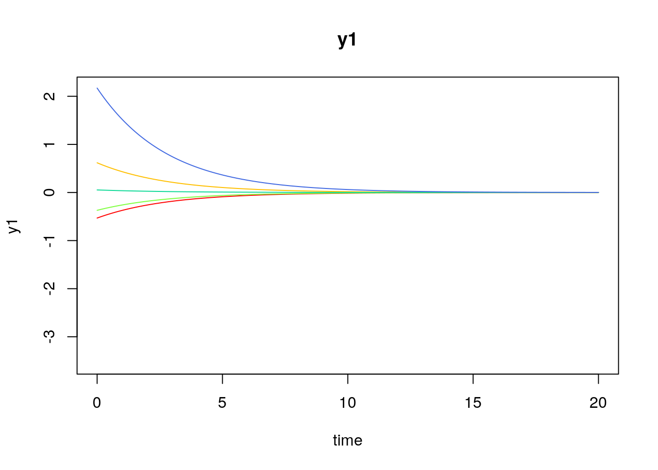
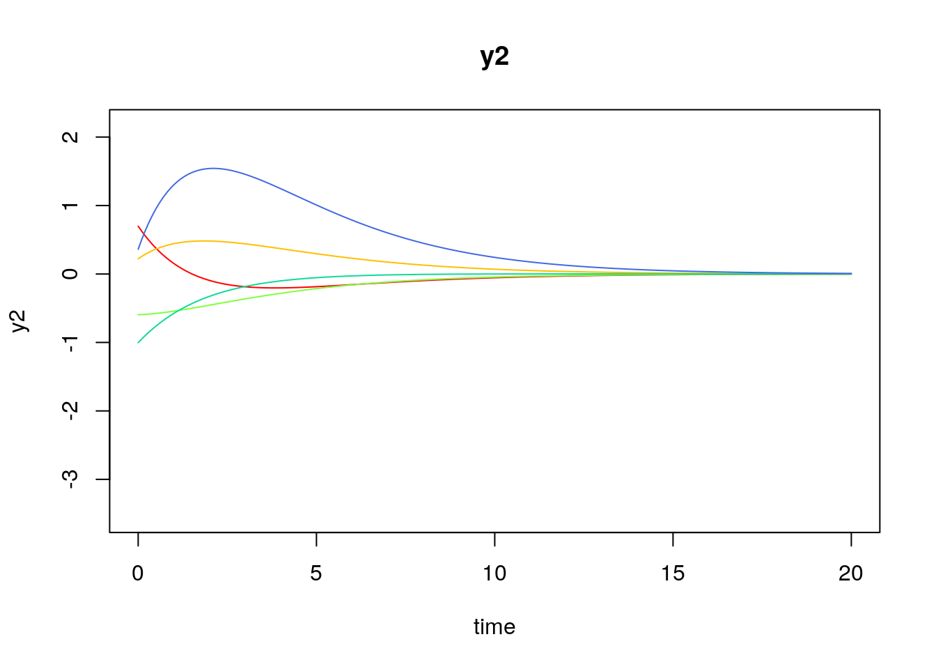
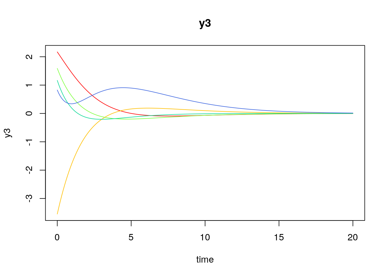
Visualizing the Dynamics Without Measurement Error and Process Noise (n = 5 with Different Initial Condition)

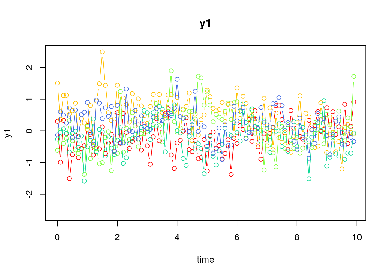
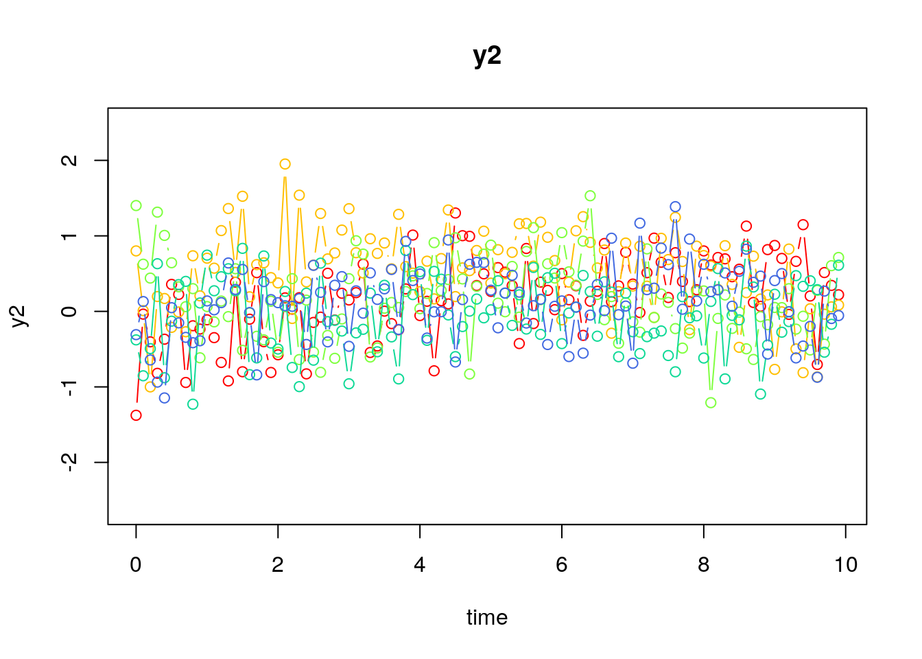
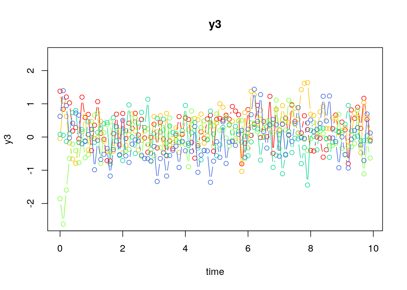
Using the SimSSMOUFixed Function from the simStateSpace Package to Simulate Data

library(simStateSpace)
sim <- SimSSMOUFixed(
  n = n,
  time = time,
  delta_t = delta_t,
  mu0 = mu0,
  sigma0_l = sigma0_l,
  mu = mu,
  phi = phi,
  sigma_l = sigma_l,
  nu = nu,
  lambda = lambda,
  theta_l = theta_l,
  type = 0
)
data <- as.data.frame(sim)
head(data)
  id time          y1          y2        y3
1  1  0.0  0.29937539 -1.37581548 1.3779071
2  1  0.1 -0.98770381 -0.03632195 0.8363080
3  1  0.2  0.33221051 -0.40321664 1.2054318
4  1  0.3 -0.09485392 -0.82030556 1.0272653
5  1  0.4 -1.50322069 -0.36841853 0.1821731
6  1  0.5 -0.75049839  0.35752476 0.2862544
summary(data)
       id         time             y1                 y2          
 Min.   :1   Min.   : 0.00   Min.   :-2.25375   Min.   :-2.75152  
 1st Qu.:2   1st Qu.:24.98   1st Qu.:-0.41569   1st Qu.:-0.47639  
 Median :3   Median :49.95   Median : 0.04509   Median : 0.08626  
 Mean   :3   Mean   :49.95   Mean   : 0.03947   Mean   : 0.05358  
 3rd Qu.:4   3rd Qu.:74.92   3rd Qu.: 0.50782   3rd Qu.: 0.61048  
 Max.   :5   Max.   :99.90   Max.   : 2.74461   Max.   : 3.02675  
       y3          
 Min.   :-2.34092  
 1st Qu.:-0.44476  
 Median : 0.02716  
 Mean   : 0.01476  
 3rd Qu.: 0.48321  
 Max.   : 2.34972  
plot(sim)

Model Fitting

Prepare Data

dynr_data <- dynr::dynr.data(
  dataframe = data,
  id = "id",
  time = "time",
  observed = c("y1", "y2", "y3")
)

Prepare Initial Condition

dynr_initial <- dynr::prep.initial(
  values.inistate = mu0,
  params.inistate = c("mu0_1_1", "mu0_2_1", "mu0_3_1"),
  values.inicov = sigma0,
  params.inicov = matrix(
    data = c(
      "sigma0_1_1", "sigma0_2_1", "sigma0_3_1",
      "sigma0_2_1", "sigma0_2_2", "sigma0_3_2",
      "sigma0_3_1", "sigma0_3_2", "sigma0_3_3"
    ),
    nrow = 3
  )
)

Prepare Measurement Model

dynr_measurement <- dynr::prep.measurement(
  values.load = diag(3),
  params.load = matrix(data = "fixed", nrow = 3, ncol = 3),
  state.names = c("eta_1", "eta_2", "eta_3"),
  obs.names = c("y1", "y2", "y3")
)

Prepare Dynamic Process

dynr_dynamics <- dynr::prep.formulaDynamics(
  formula = list(
    eta_1 ~ (phi_1_1 * (eta_1 - mu_1_1)) + (phi_1_2 * (eta_2 - mu_2_1)) + (phi_1_3 * (eta_3 - mu_3_1)),
    eta_2 ~ (phi_2_1 * (eta_1 - mu_1_1)) + (phi_2_2 * (eta_2 - mu_2_1)) + (phi_2_3 * (eta_3 - mu_3_1)),
    eta_3 ~ (phi_3_1 * (eta_1 - mu_1_1)) + (phi_3_2 * (eta_2 - mu_2_1)) + (phi_3_3 * (eta_3 - mu_3_1))
  ),
  startval = c(
    mu_1_1 = mu[1], mu_2_1 = mu[2], mu_3_1 = mu[3],
    phi_1_1 = phi[1, 1], phi_1_2 = phi[1, 2], phi_1_3 = phi[1, 3],
    phi_2_1 = phi[2, 1], phi_2_2 = phi[2, 2], phi_2_3 = phi[2, 3],
    phi_3_1 = phi[3, 1], phi_3_2 = phi[3, 2], phi_3_3 = phi[3, 3]
  ),
  isContinuousTime = TRUE
)

Prepare Process Noise

dynr_noise <- dynr::prep.noise(
  values.latent = sigma,
  params.latent = matrix(
    data = c(
      "sigma_1_1", "sigma_2_1", "sigma_3_1",
      "sigma_2_1", "sigma_2_2", "sigma_3_2",
      "sigma_3_1", "sigma_3_2", "sigma_3_3"
    ),
    nrow = 3
  ),
  values.observed = theta,
  params.observed = matrix(
    data = c(
      "theta_1_1", "fixed", "fixed",
      "fixed", "theta_2_2", "fixed",
      "fixed", "fixed", "theta_3_3"
    ),
    nrow = 3
  )
)

Prepare the Model

model <- dynr::dynr.model(
  data = dynr_data,
  initial = dynr_initial,
  measurement = dynr_measurement,
  dynamics = dynr_dynamics,
  noise = dynr_noise,
  outfile = "ou.c"
)

Add lower and upper bounds to aid in the optimization.

model$lb[
  c(
    "phi_1_1",
    "phi_1_2",
    "phi_1_3",
    "phi_2_1",
    "phi_2_2",
    "phi_2_3",
    "phi_3_1",
    "phi_3_2",
    "phi_3_3"
  )
] <- -1.5
model$ub[
  c(
    "phi_1_1",
    "phi_1_2",
    "phi_1_3",
    "phi_2_1",
    "phi_2_2",
    "phi_2_3",
    "phi_3_1",
    "phi_3_2",
    "phi_3_3"
  )
] <- +1.5

Fit the Model

results <- dynr::dynr.cook(
  model,
  debug_flag = TRUE,
  verbose = FALSE
)
[1] "Get ready!!!!"
using C compiler: ‘gcc (Ubuntu 13.3.0-6ubuntu2~24.04) 13.3.0’
Optimization function called.
Starting Hessian calculation ...
Finished Hessian calculation.
Original exit flag:  3 
Modified exit flag:  3 
Optimization terminated successfully: ftol_rel or ftol_abs was reached. 
Original fitted parameters:  0.05480875 0.0970006 0.04993973 -0.434506 
0.02467277 -0.05454905 0.8417982 -0.6017518 0.1099265 -0.3702948 0.6609449 
-0.6606183 -1.381888 0.08161089 -0.2479494 -2.480951 0.1751864 -2.810068 
-1.625097 -1.682562 -1.597112 -0.3660337 -0.4092527 0.2149727 -0.7538976 
0.6368556 0.4928618 -0.5914103 0.6108847 -2.103637 

Transformed fitted parameters:  0.05480875 0.0970006 0.04993973 -0.434506 
0.02467277 -0.05454905 0.8417982 -0.6017518 0.1099265 -0.3702948 0.6609449 
-0.6606183 0.2511041 0.02049283 -0.0622611 0.08533609 0.009575553 0.07820615 
0.1968925 0.1858971 0.2024804 -0.3660337 -0.4092527 0.2149727 0.470529 
0.2996591 0.2319058 0.7443856 0.4858433 0.4428818 

Doing end processing
Successful trial
Total Time: 4.105517 
Backend Time: 4.097889 

Summary

summary(results)
Coefficients:
            Estimate Std. Error t value  ci.lower  ci.upper Pr(>|t|)    
mu_1_1      0.054809   0.051341   1.068 -0.045818  0.155436   0.1429    
mu_2_1      0.097001   0.086113   1.126 -0.071777  0.265778   0.1300    
mu_3_1      0.049940   0.057135   0.874 -0.062042  0.161922   0.1911    
phi_1_1    -0.434506   0.180354  -2.409 -0.787994 -0.081018   0.0080 ** 
phi_1_2     0.024673   0.154258   0.160 -0.277668  0.327013   0.4365    
phi_1_3    -0.054549   0.126095  -0.433 -0.301690  0.192592   0.3327    
phi_2_1     0.841798   0.116934   7.199  0.612611  1.070985   <2e-16 ***
phi_2_2    -0.601752   0.102169  -5.890 -0.802000 -0.401504   <2e-16 ***
phi_2_3     0.109926   0.083850   1.311 -0.054416  0.274269   0.0950 .  
phi_3_1    -0.370295   0.114555  -3.232 -0.594819 -0.145771   0.0006 ***
phi_3_2     0.660945   0.099134   6.667  0.466647  0.855243   <2e-16 ***
phi_3_3    -0.660618   0.081176  -8.138 -0.819720 -0.501517   <2e-16 ***
sigma_1_1   0.251104   0.031869   7.879  0.188642  0.313566   <2e-16 ***
sigma_2_1   0.020493   0.012759   1.606 -0.004513  0.045499   0.0541 .  
sigma_3_1  -0.062261   0.012982  -4.796 -0.087706 -0.036816   <2e-16 ***
sigma_2_2   0.085336   0.010363   8.234  0.065024  0.105648   <2e-16 ***
sigma_3_2   0.009576   0.006803   1.408 -0.003758  0.022909   0.0797 .  
sigma_3_3   0.078206   0.009743   8.027  0.059110  0.097303   <2e-16 ***
theta_1_1   0.196892   0.005250  37.504  0.186603  0.207182   <2e-16 ***
theta_2_2   0.185897   0.004255  43.687  0.177557  0.194237   <2e-16 ***
theta_3_3   0.202480   0.004592  44.090  0.193479  0.211481   <2e-16 ***
mu0_1_1    -0.366034   0.327590  -1.117 -1.008099  0.276031   0.1319    
mu0_2_1    -0.409253   0.397704  -1.029 -1.188738  0.370233   0.1518    
mu0_3_1     0.214973   0.314431   0.684 -0.401300  0.831246   0.2471    
sigma0_1_1  0.470529   0.340595   1.381 -0.197025  1.138083   0.0836 .  
sigma0_2_1  0.299659   0.323106   0.927 -0.333617  0.932935   0.1769    
sigma0_3_1  0.231906   0.254674   0.911 -0.267246  0.731058   0.1813    
sigma0_2_2  0.744386   0.505722   1.472 -0.246811  1.735582   0.0706 .  
sigma0_3_2  0.485843   0.352649   1.378 -0.205336  1.177023   0.0842 .  
sigma0_3_3  0.442882   0.313556   1.412 -0.171676  1.057439   0.0789 .  
---
Signif. codes:  0 '***' 0.001 '**' 0.01 '*' 0.05 '.' 0.1 ' ' 1

-2 log-likelihood value at convergence = 21202.41
AIC = 21262.41
BIC = 21457.92
[1] -0.3660337 -0.4092527  0.2149727

Parameter Estimates

mu_hat
[1] 0.05480875 0.09700060 0.04993973
phi_hat
           [,1]        [,2]        [,3]
[1,] -0.4345060  0.02467277 -0.05454905
[2,]  0.8417982 -0.60175178  0.10992650
[3,] -0.3702948  0.66094491 -0.66061828
sigma_hat
            [,1]        [,2]         [,3]
[1,]  0.25110408 0.020492828 -0.062261099
[2,]  0.02049283 0.085336089  0.009575553
[3,] -0.06226110 0.009575553  0.078206146
mu0_hat
[1] -0.3660337 -0.4092527  0.2149727
sigma0_hat
          [,1]      [,2]      [,3]
[1,] 0.4705290 0.2996591 0.2319058
[2,] 0.2996591 0.7443856 0.4858433
[3,] 0.2319058 0.4858433 0.4428818
beta_var1_hat <- expm::expm(phi_hat)
beta_var1_hat
            [,1]        [,2]        [,3]
[1,]  0.65704464 0.004621693 -0.03138432
[2,]  0.49886539 0.570658931  0.04636742
[3,] -0.05872866 0.355366244  0.53861155