The following is a simple benchmark comparing the computational requirements of the methods to generate confidence intervals for the indirect effect with missing observations. We will use the generated data in the Data Generation article.
In this benchmark, we compare the following methods
- Monte Carlo method using full-information maximum likelihood
(
MCML()), - Monte Carlo method using multiple imputation
(
MCMI()), - full-information maximum likelihood nested within nonparametric
bootstrap (
NBML()), - multiple imputation nested within nonparametric bootstrap
(
NBMI()) - nonparametric bootstrap nested within multiple imputation
(
MINB())
Arguments
| Variables | Values | Notes |
|---|---|---|
| m | 100 | Number of imputations. |
| R | 5000 | Number of Monte Carlo replications. |
| B | 5000 | Number of bootstrap samples. |
| mplus_bin | “/opt/mplusdemo/mpdemo” | Path to Mplus binary. |
NOTE: If you are using
manmcmedmiss-rockerormanmcmedmiss.sifdescribed in the Containers article, setmplus_bin = "mpdemo".
Parameters
| Variable | Value | Notes |
|---|---|---|
| n | 50 | \(n\) |
| tauprime | 0.14142135623731 | \(\tau^{\prime}\) |
| alpha | 0.714074191775111 | \(\alpha\) |
| beta | 0.714074191775111 | \(\beta\) |
Data
Amputation
Generate sample data with missing values using the multivariate amputation approach proposed by Schouten et al. (2018).
data_missing <- AmputeData(
  data_complete,
  mech = "MAR",
  prop = 0.10
)
Imputation
Perform multiple imputation following Asparouhov and Muthen (2010)
using Mplus.
data_mi <- ImputeData(
  data_missing,
  m = m,
  mplus_bin = mplus_bin
)
Maximum Likelihood
Missing Data
Parameters of the simple mediation model are estimated using full-information maximum likelihood to handle missing data.
fit_ml <- FitModelML(
  data_missing,
  mplus_bin = mplus_bin
)
Multiple Imputation
Parameters of the simple mediation model are estimated using maximum likelihood for each of the imputed data sets. The parameter estimates and their sampling covariance matrix are pooled.
fit_mi <- FitModelMI(
  data_mi,
  mplus_bin = mplus_bin
)Summary of Benchmark Results
summary(benchmark, unit = "ms")
#>   expr          min           lq         mean       median           uq
#> 1 MCML     18.73027     34.62104     48.37869     46.02422 5.337519e+01
#> 2 MCMI     32.08413     34.56102     68.64550     61.40423 1.054957e+02
#> 3 NBML   1779.85401   1995.39254   2686.87359   2700.63207 3.396238e+03
#> 4 NBMI 626443.36697 787734.54704 907889.17563 818272.44441 1.090418e+06
#> 5 MINB  43613.55303  46511.95203  60975.13838  48293.08648 8.038919e+04
#>            max neval cld
#> 1     101.9532    10  a
#> 2     123.1622    10  a
#> 3    3541.1389    10  a
#> 4 1263013.0070    10   b
#> 5   92118.3821    10  a
Summary of Benchmark Results Relative to the Fastest Method
summary(benchmark, unit = "relative")
#>   expr          min           lq        mean       median           uq
#> 1 MCML     1.000000 1.000000e+00     1.00000     1.000000     1.000000
#> 2 MCMI     1.712956 9.982665e-01     1.41892     1.334172     1.976494
#> 3 NBML    95.025549 5.763526e+01    55.53837    58.678492    63.629527
#> 4 NBMI 33445.510068 2.275306e+04 18766.30431 17779.168542 20429.300198
#> 5 MINB  2328.506620 1.343459e+03  1260.37190  1049.297126  1506.115228
#>            max neval cld
#> 1     1.000000    10  a
#> 2     1.208027    10  a
#> 3    34.732974    10  a
#> 4 12388.160554    10   b
#> 5   903.535673    10  a
Plot
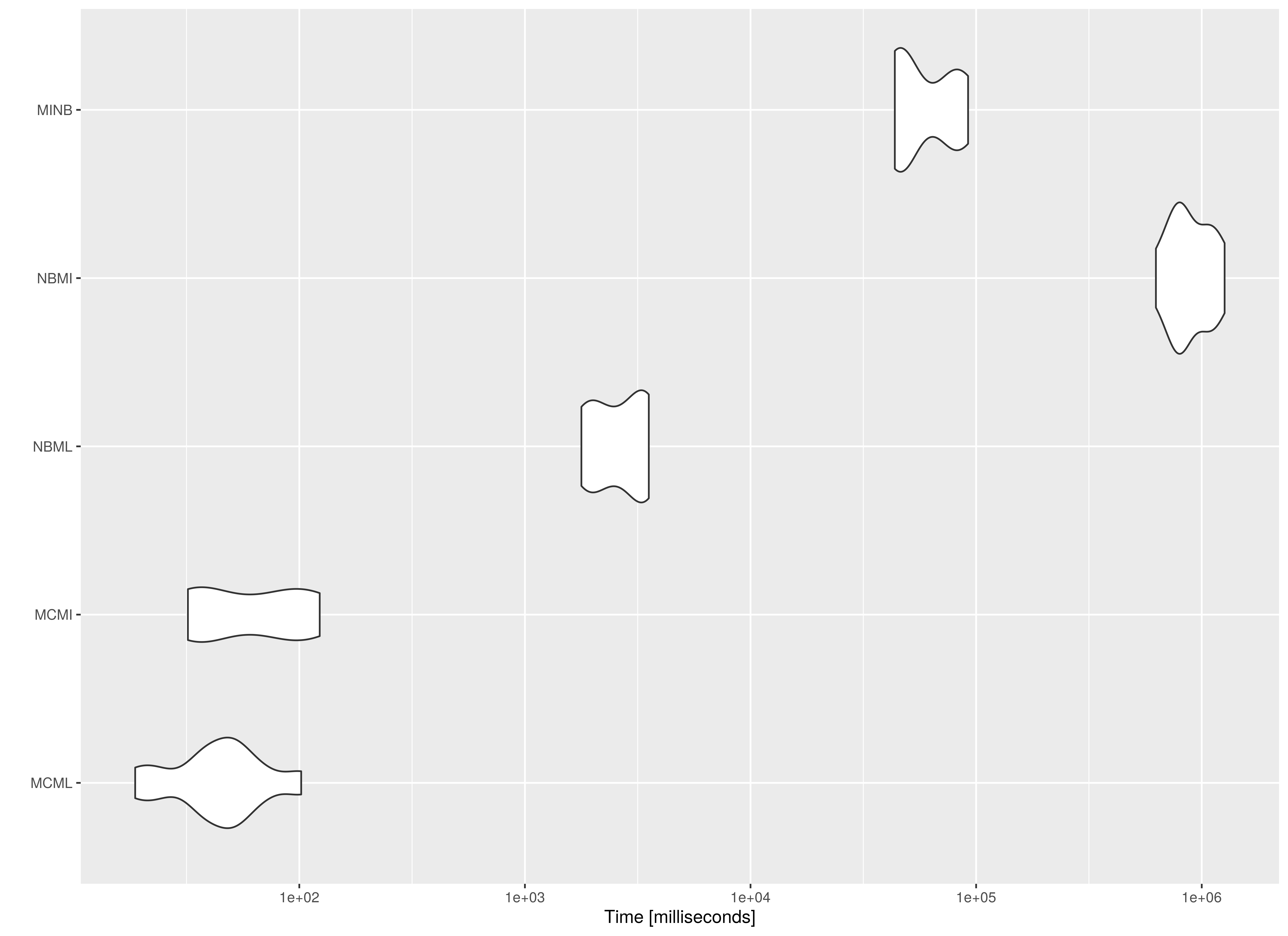
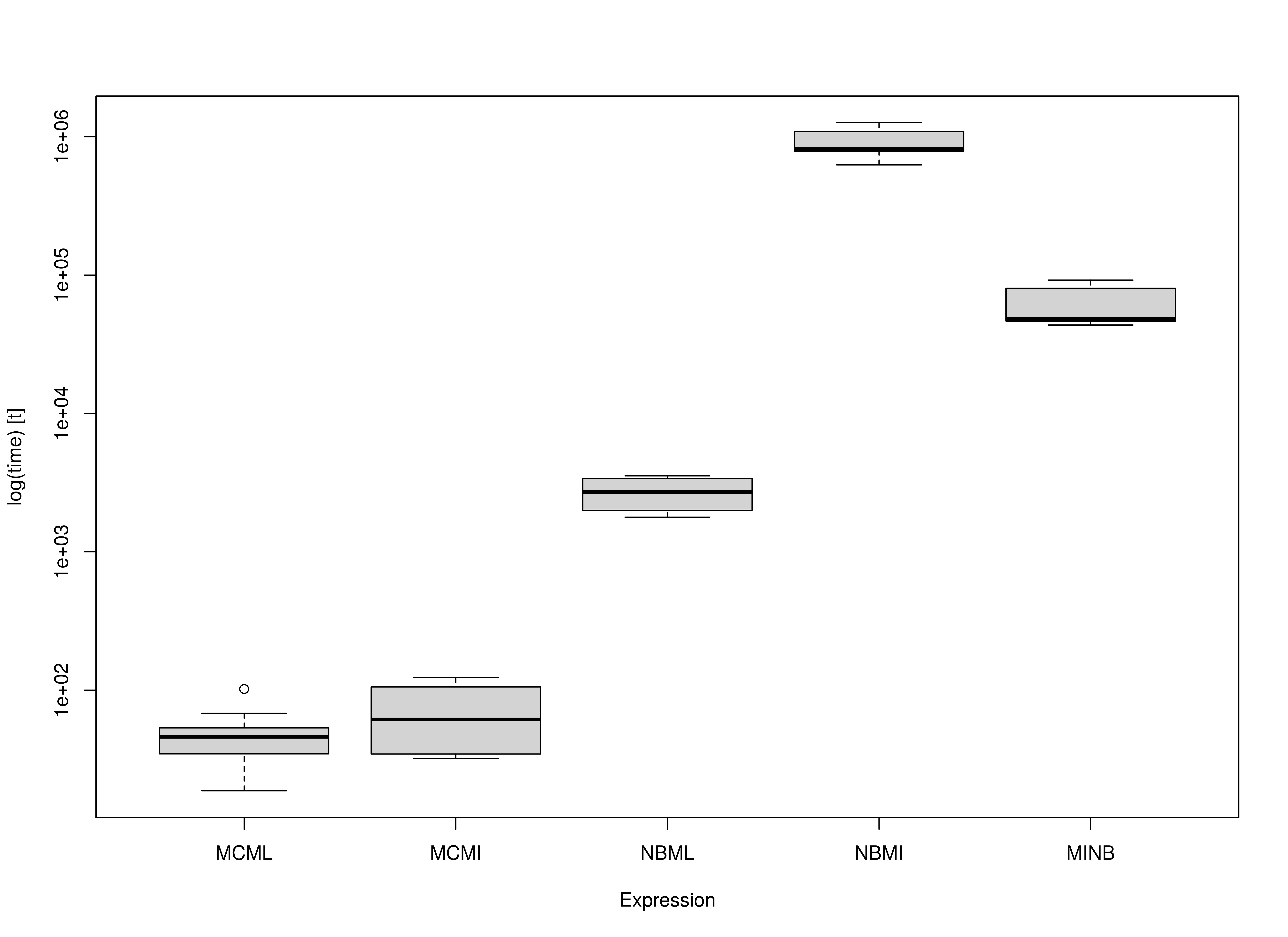
The MC approaches are faster compared to their
NB counterparts. Note the increasing model complexity will
increase the computational cost of NB. However, for
MC, model complexity will not increase the computational
cost of the simulation stage. For example, MI estimates are
more computationally intensive than ML estimates. This
results in a large difference between NBML and the two
NB methods using MI, that is,
NBMI and MINB. Note that MINB is
faster than NBMI as expected but it is still significantly
slower than the MC approaches.
However, if we perform the model fitting step outside the benchmark
calculation, the speed of MCML and MCMI will
be virtually identical. In this implementation, however,
MCMI will be a little bit slower than MCML
because it generates two sets of confidence intervals (vcov
and vcov_tilde) while MCML generates a single
set. Since MC relies on a single estimate of the parameters
and the sampling covariance matrix, it is suited for more complex
models.
NOTE: Note that since
NBonly needs point estimates, a closed form solution of the indirect effect is used inNBMIandMINB. When optimization is used to estimate parameters in the context of structural equation modeling,NBMIandMINBwill be significantly slower.