Scatter Plots - Strong Coupling

Ivan Jacob Agaloos Pesigan

library(manCTMed)

Population Total, Direct, and Indirect Effects

Total, direct, and indirect effects for the drift matrix

$$\begin{equation} \left( \begin{array}{ccc} −0.714 & 0 & 0 \\ 1.542 & −1.022 & 0 \\ −0.900 & 1.458 & −1.386 \\ \end{array} \right) \end{equation}$$

FigPlotEffects(dynamics = 1)
#> 
#> phi:
#>        x      m      y
#> x -0.714  0.000  0.000
#> m  1.542 -1.022  0.000
#> y -0.900  1.458 -1.386

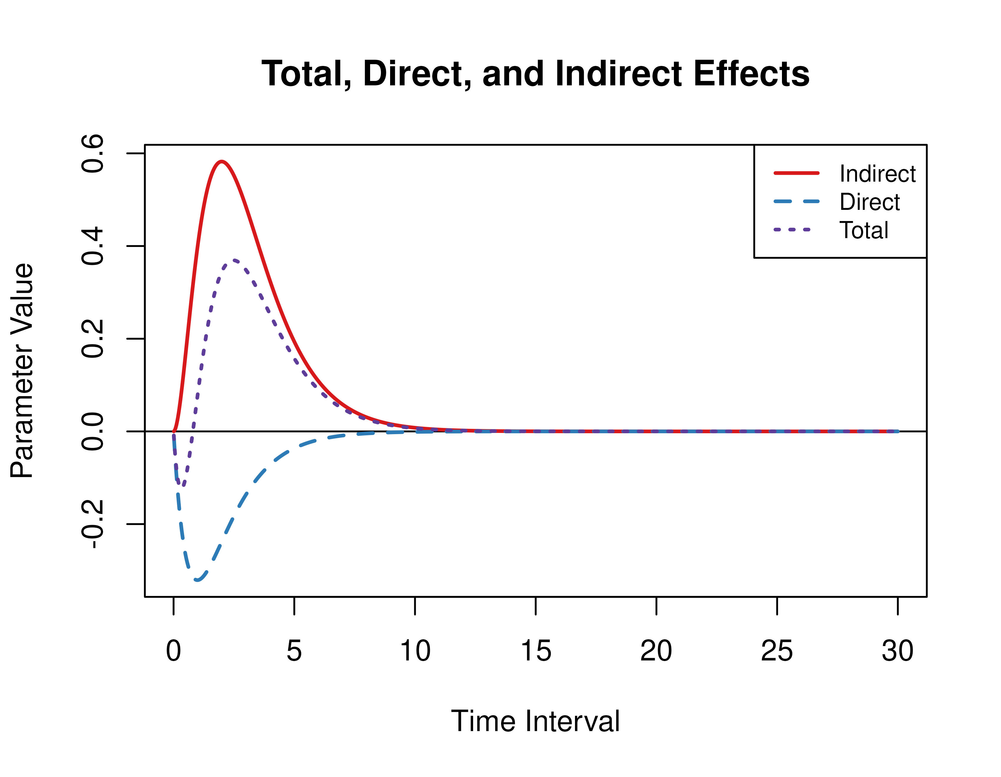
Standardized total, direct, and indirect effects for the drift matrix $$\begin{equation} \left( \begin{array}{ccc} −0.714 & 0 & 0 \\ 1.542 & −1.022 & 0 \\ −0.900 & 1.458 & −1.386 \\ \end{array} \right) \end{equation}$$ and process noise covariance matrix $$\begin{equation} \left( \begin{array}{ccc} 0.4891 & 0.0440 & -0.1001 \\ 0.0440 & 0.1414 & 0.0308 \\ -0.1001 & 0.0308 & 0.1511 \\ \end{array} \right) \end{equation}$$

FigPlotEffects(dynamics = 1, std = TRUE)
#> 
#> phi:
#>        x      m      y
#> x -0.714  0.000  0.000
#> m  1.542 -1.022  0.000
#> y -0.900  1.458 -1.386
#> 
#> sigma:
#>             [,1]       [,2]        [,3]
#> [1,]  0.24455556 0.02201587 -0.05004762
#> [2,]  0.02201587 0.07067800  0.01539456
#> [3,] -0.05004762 0.01539456  0.07553061

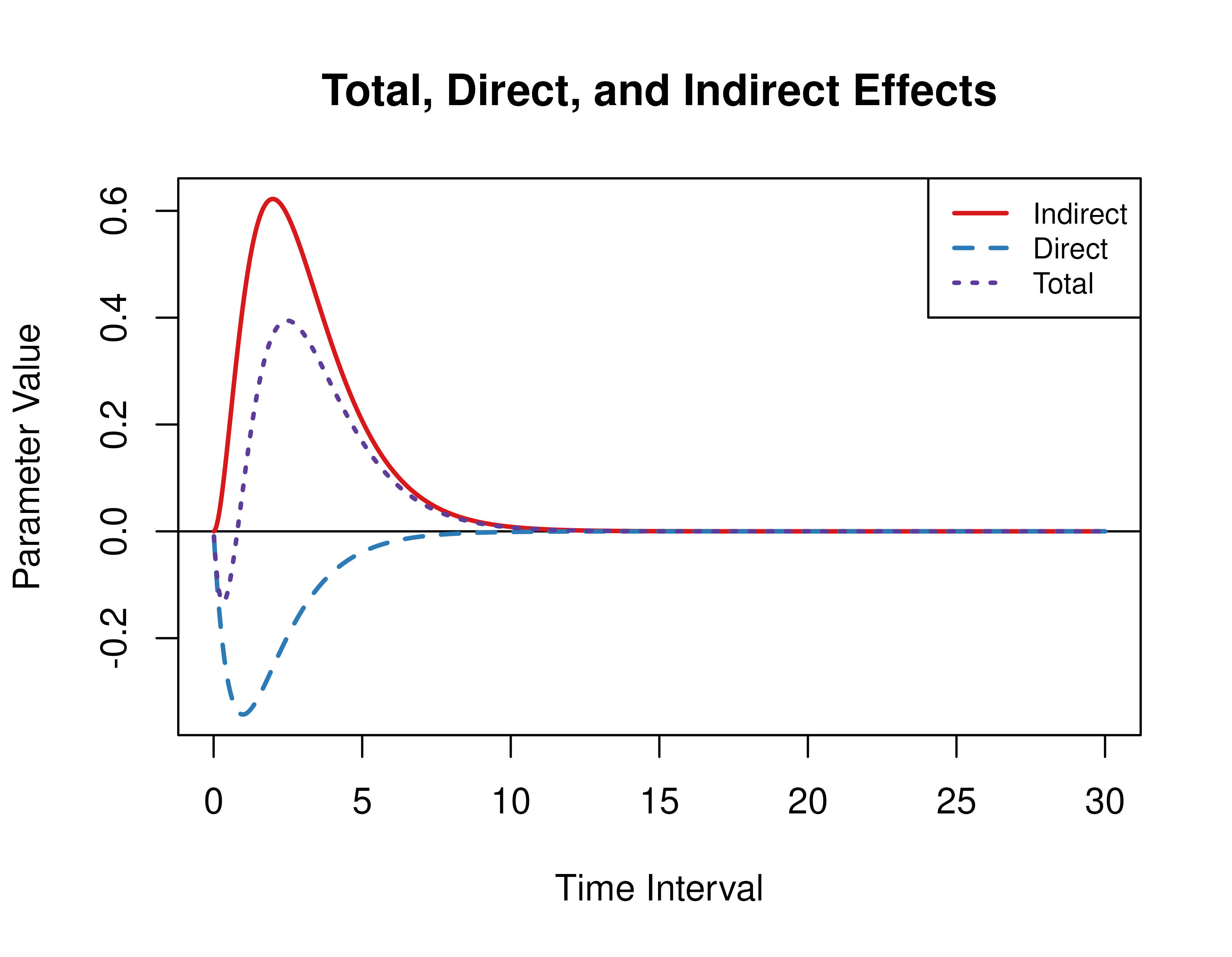
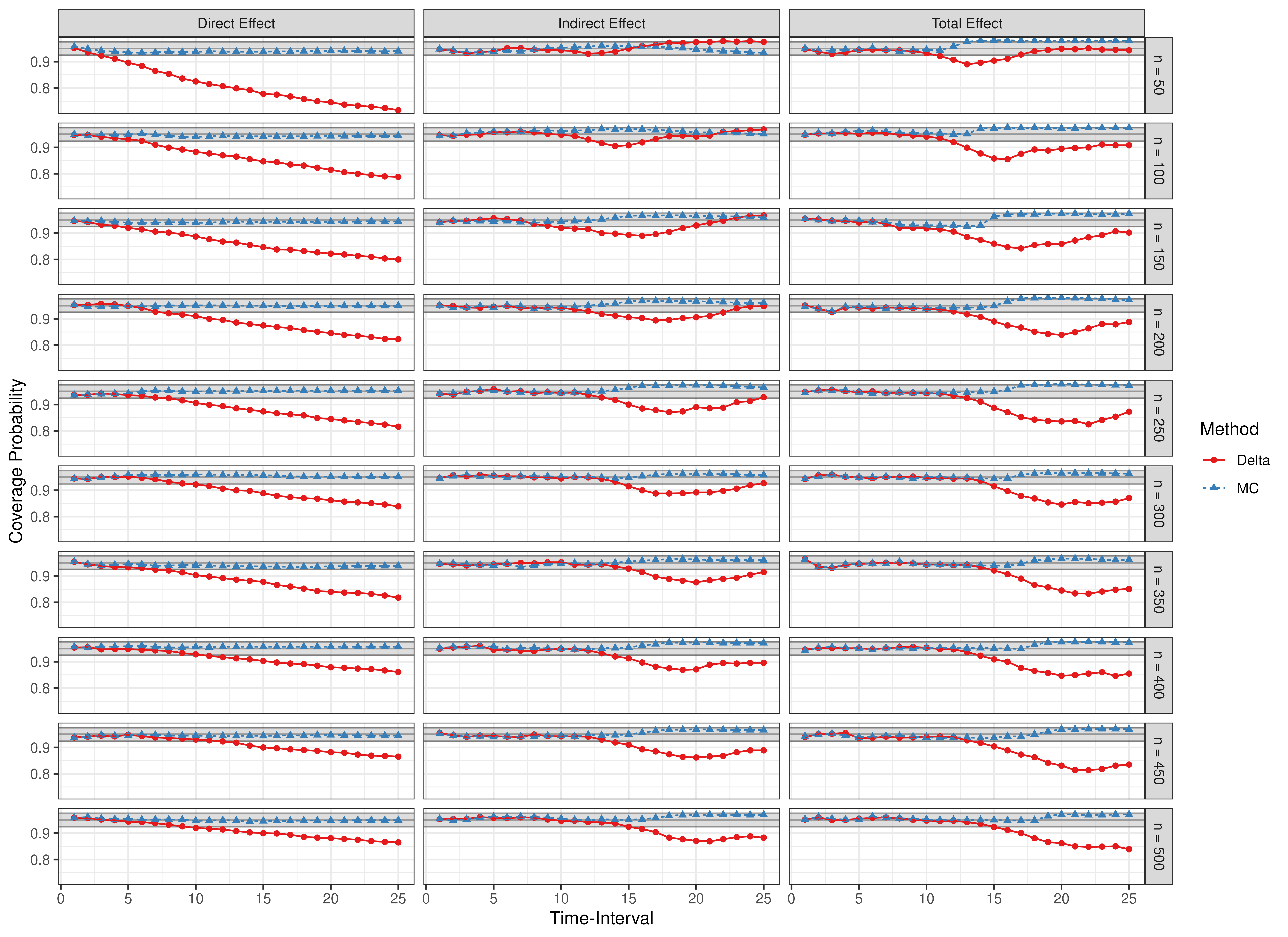
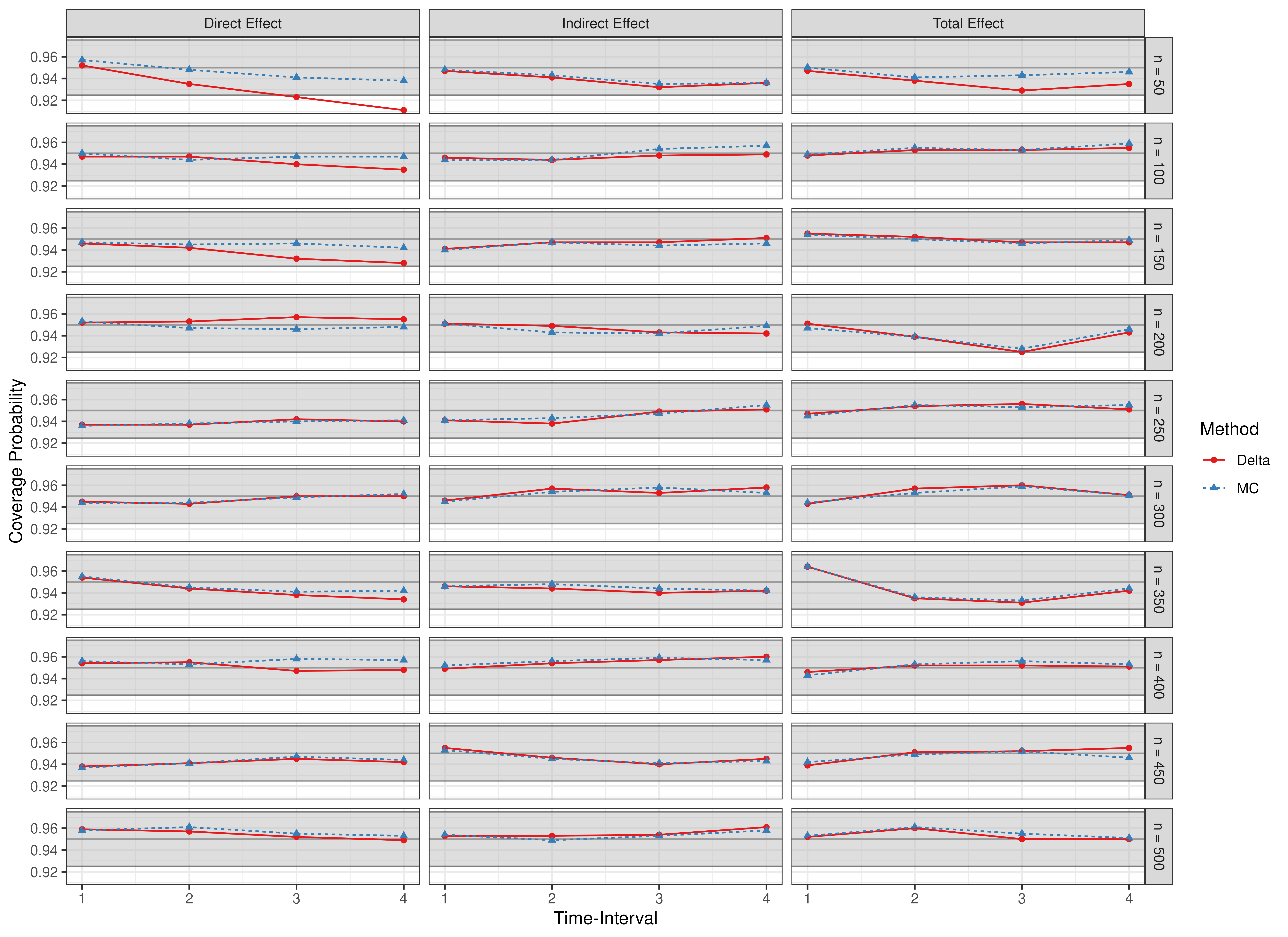
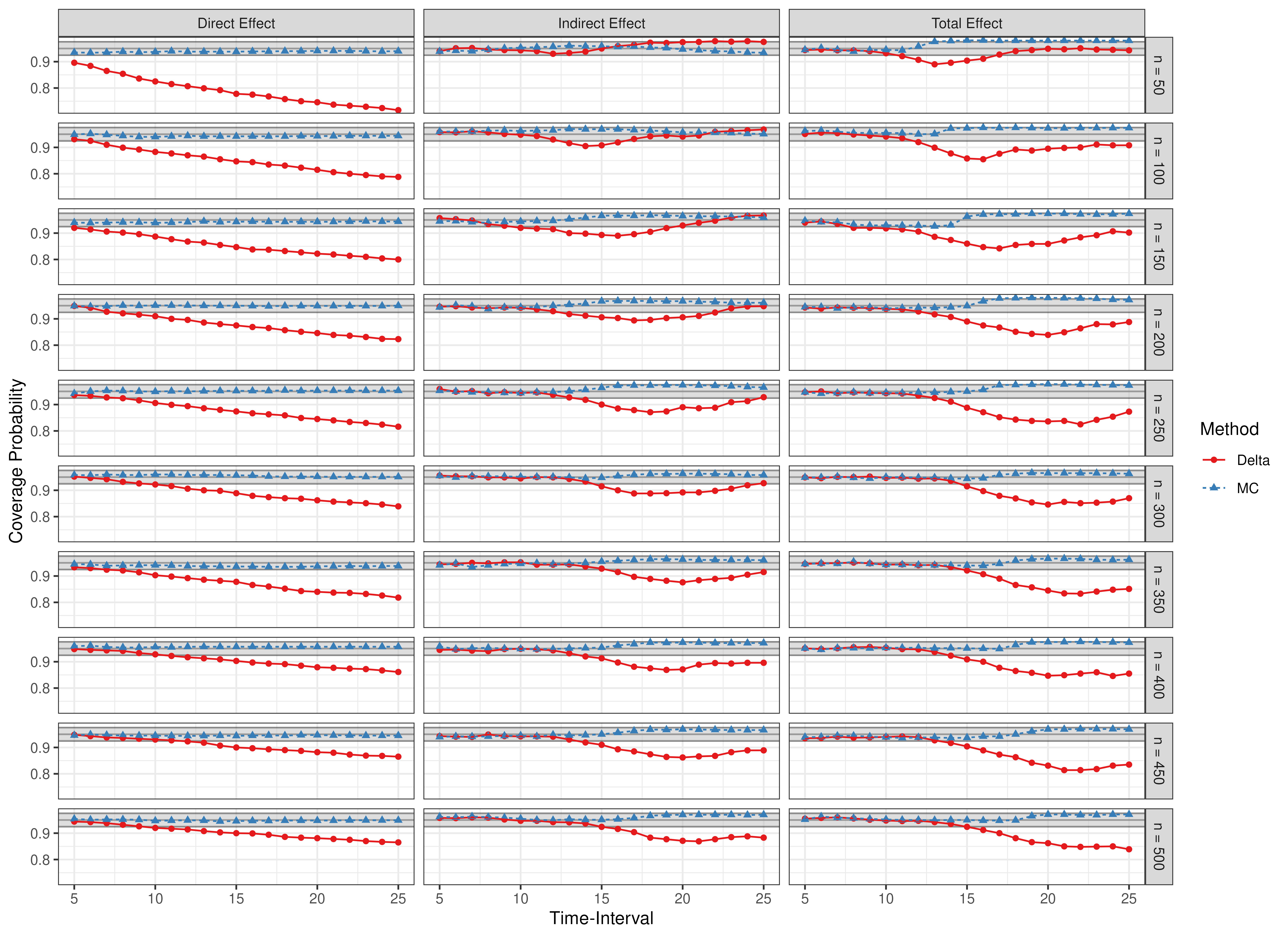
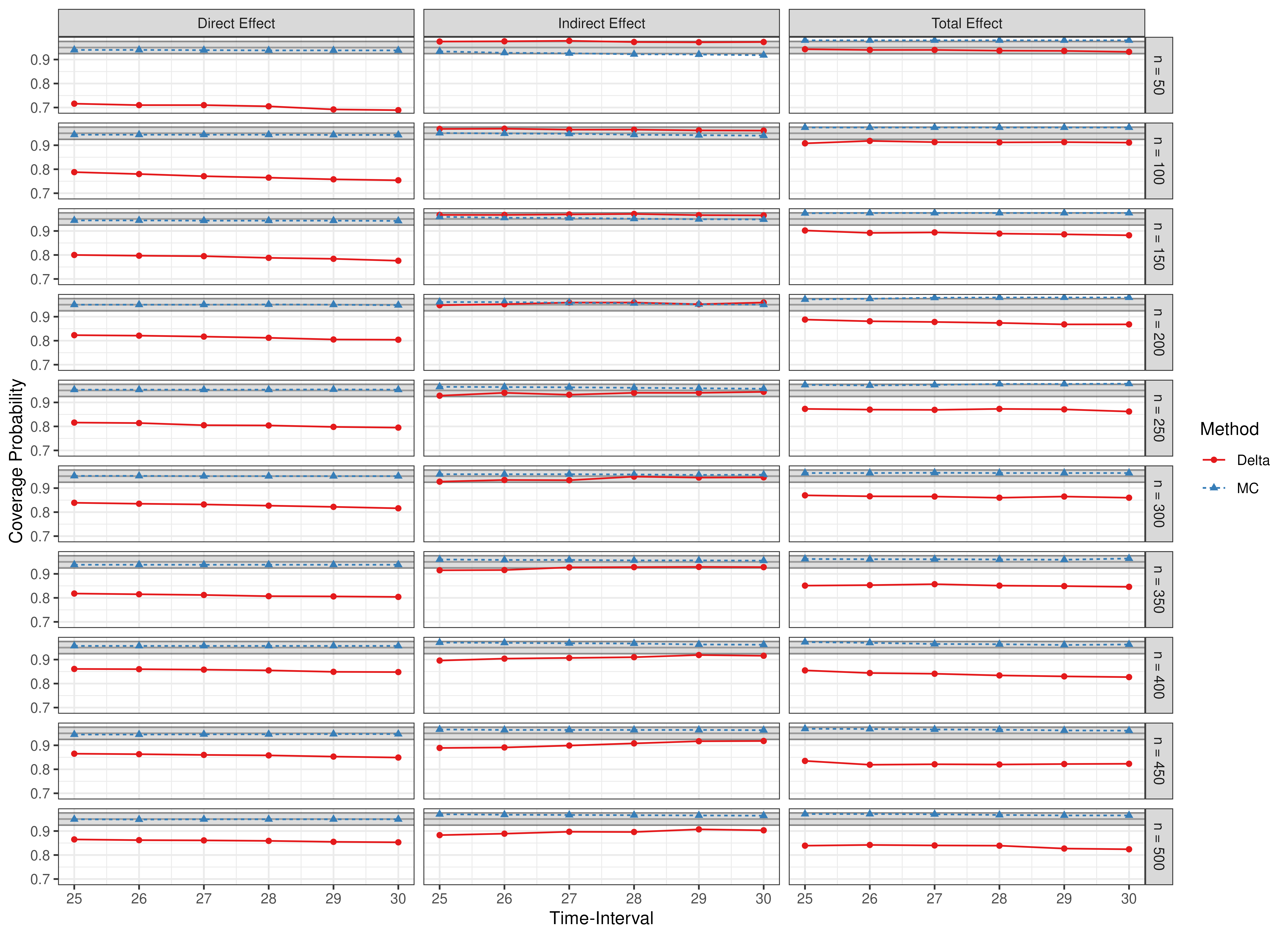
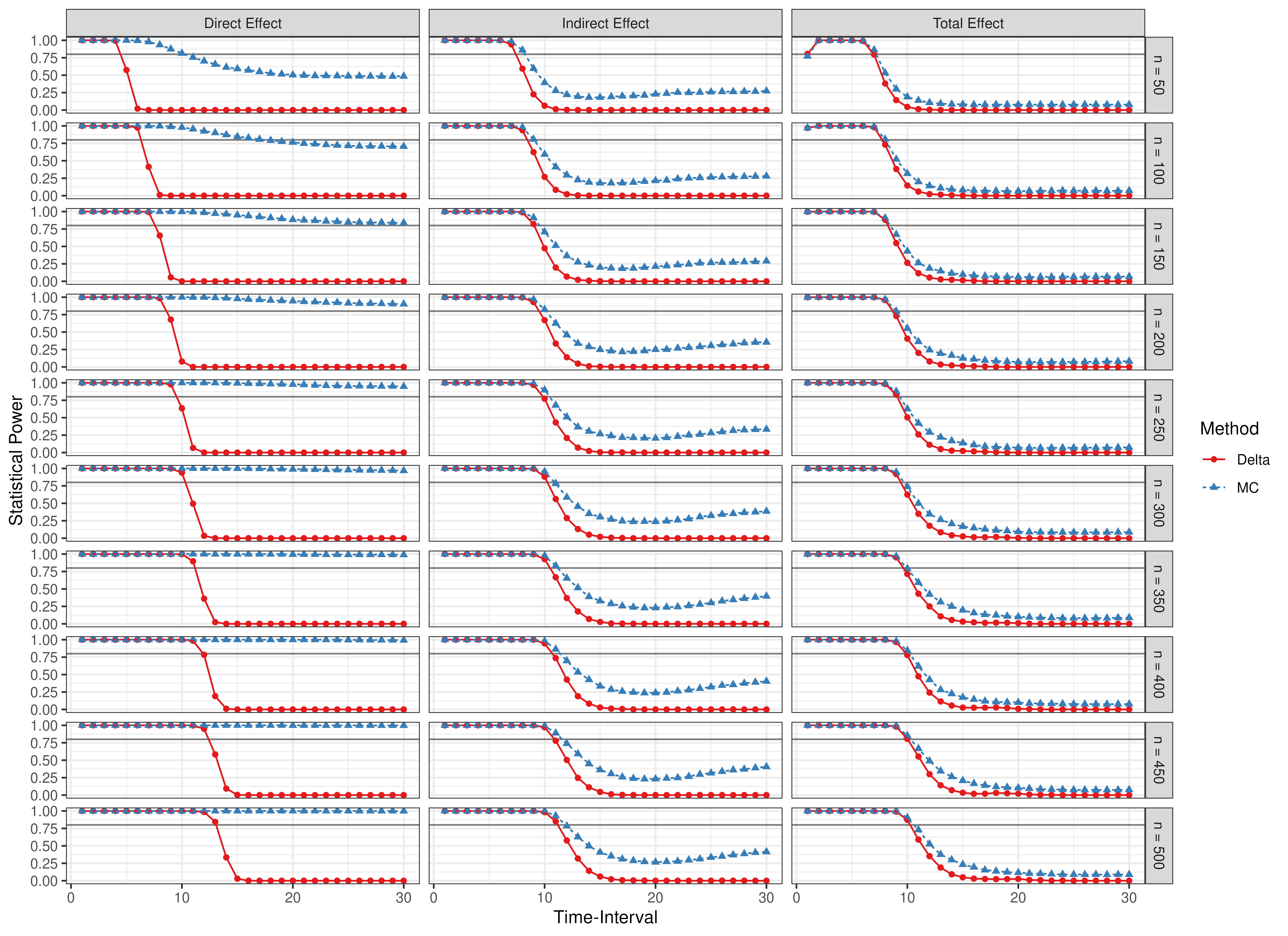
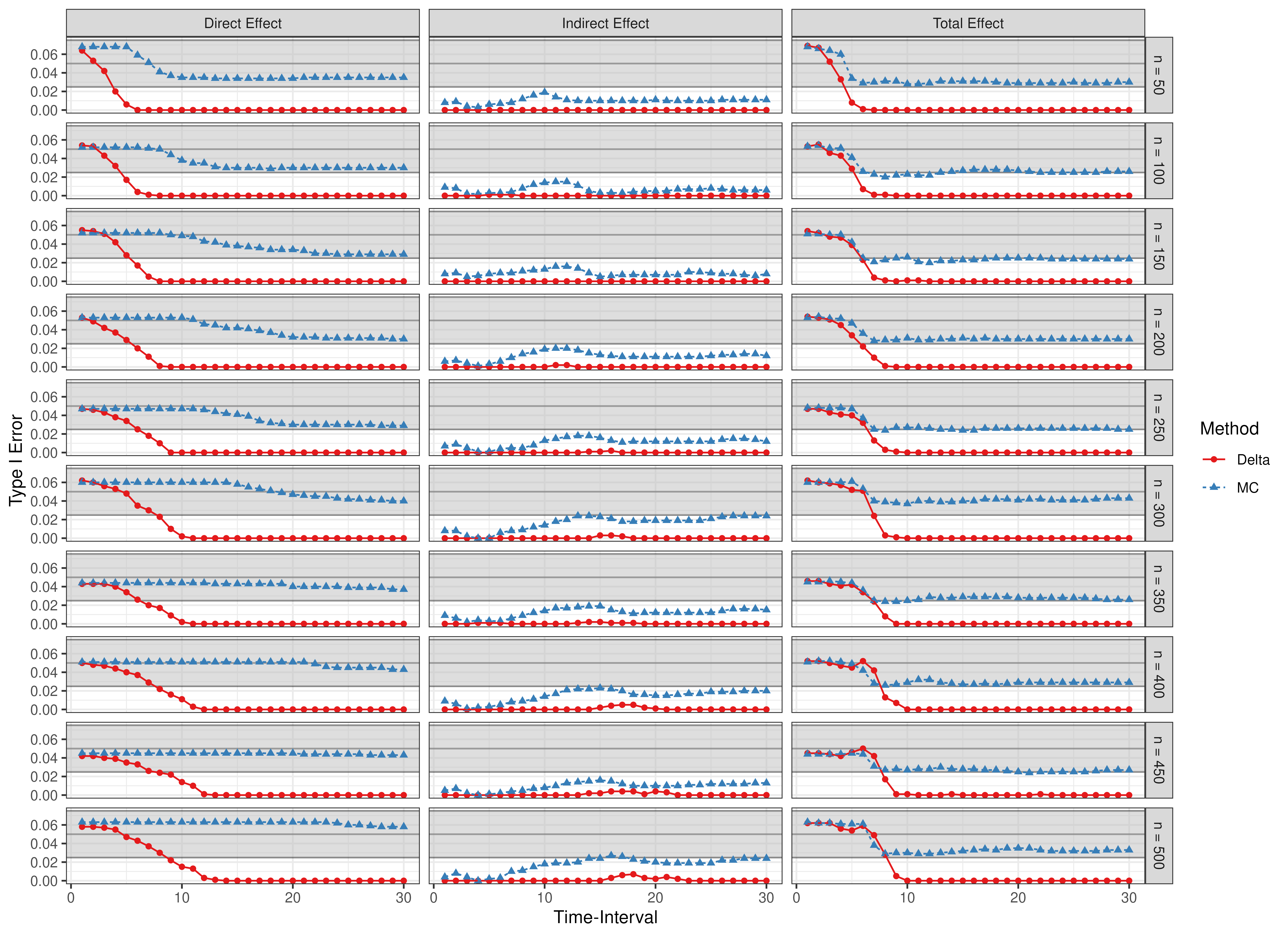
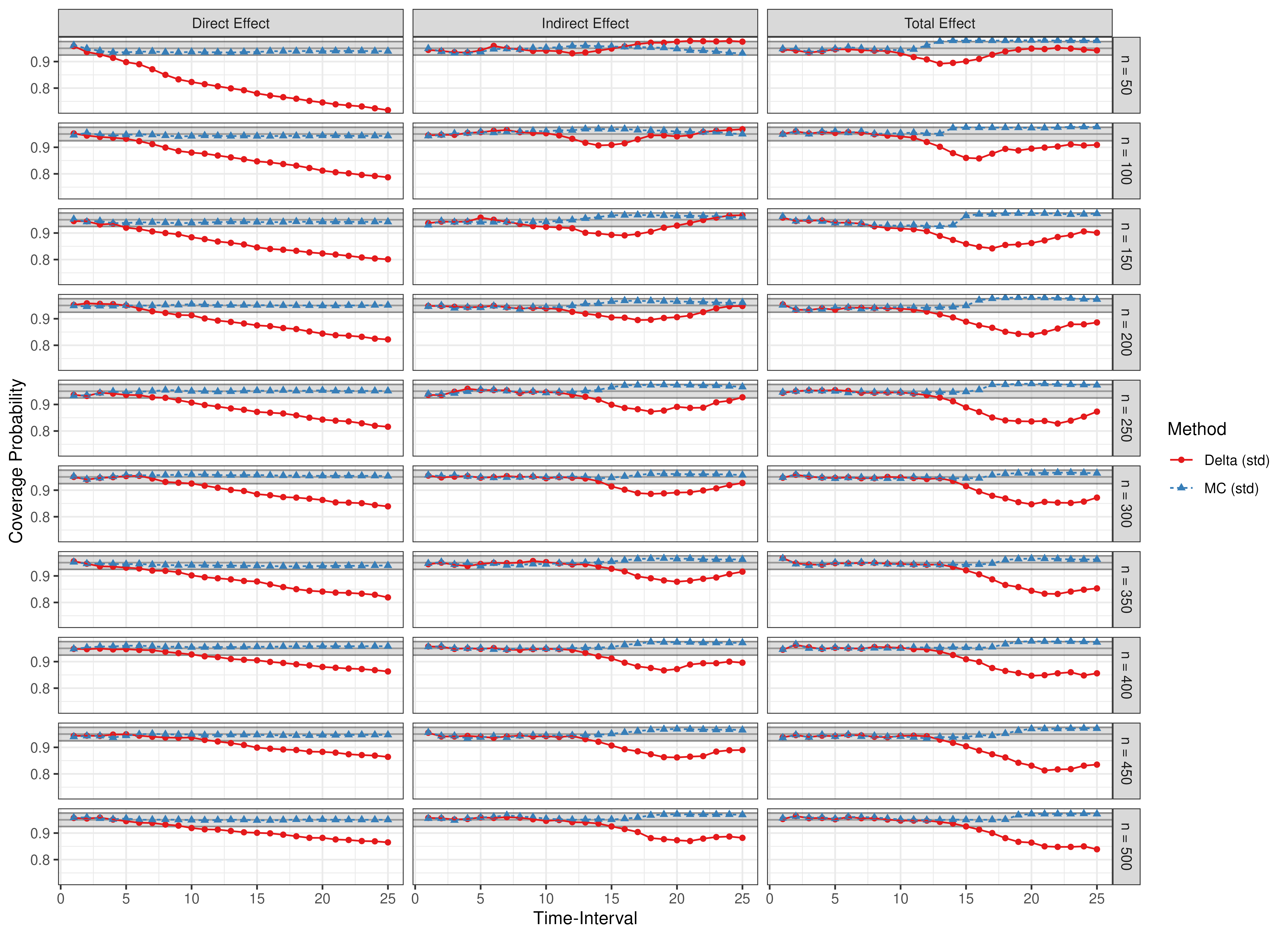
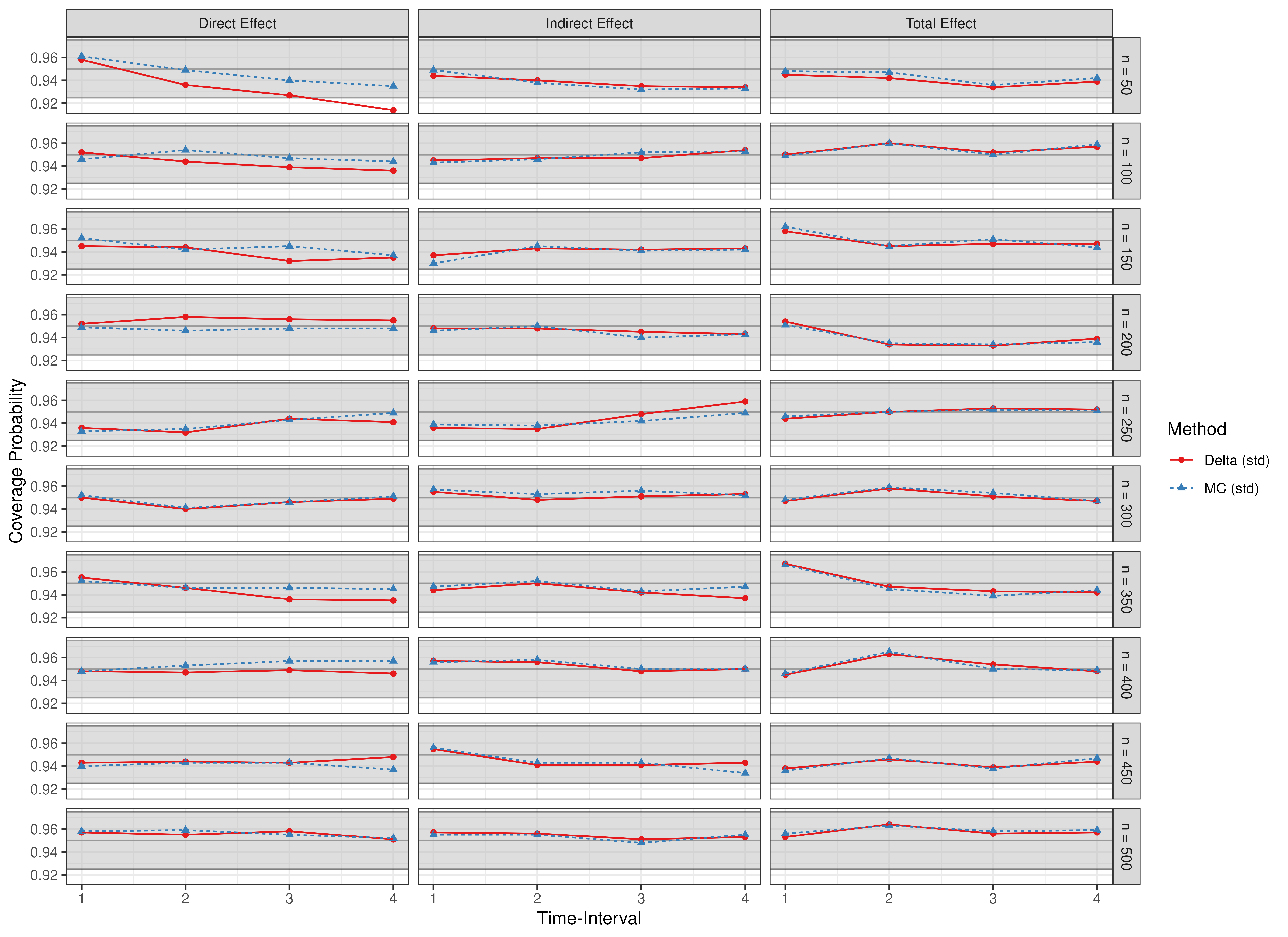
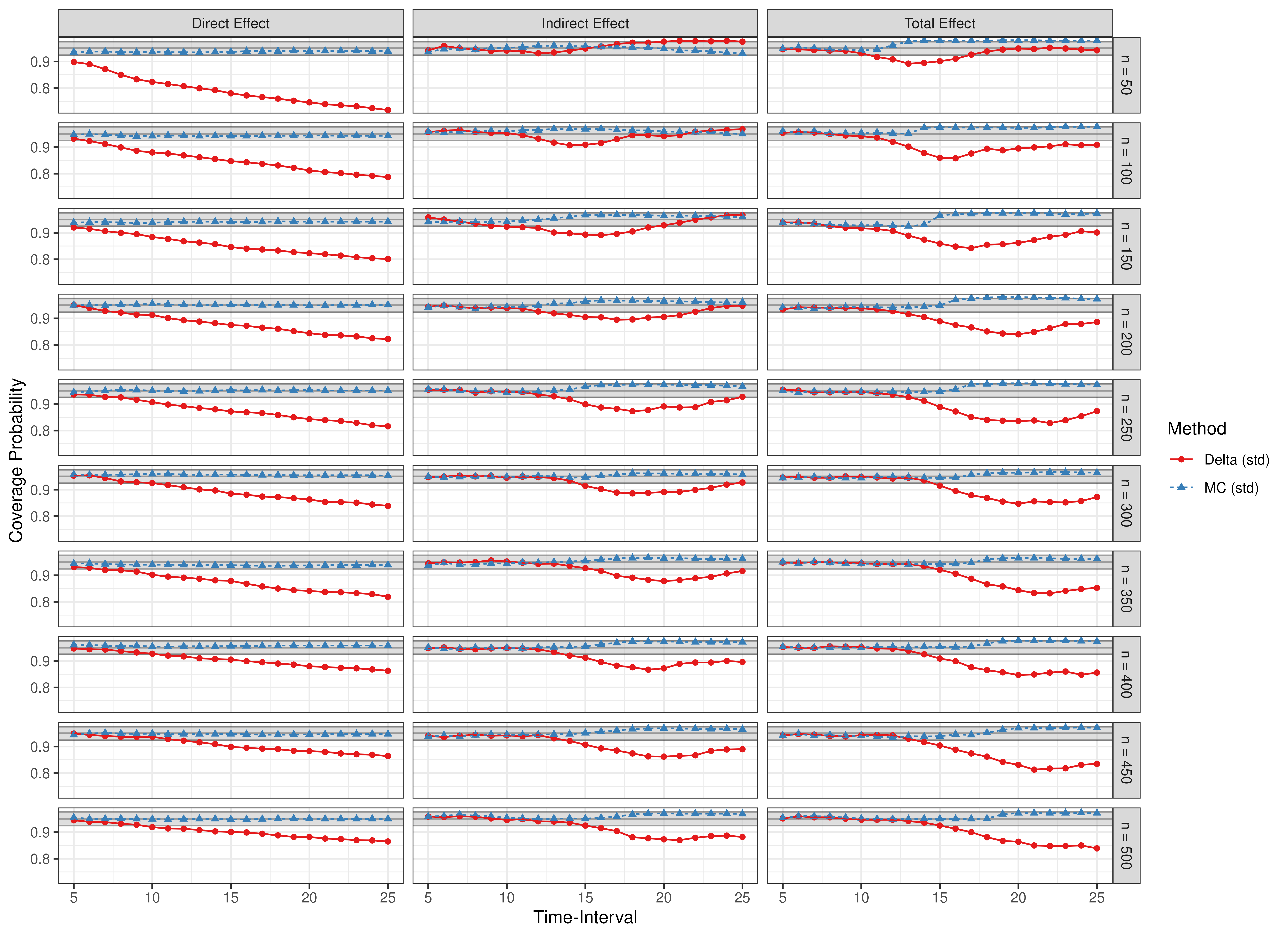
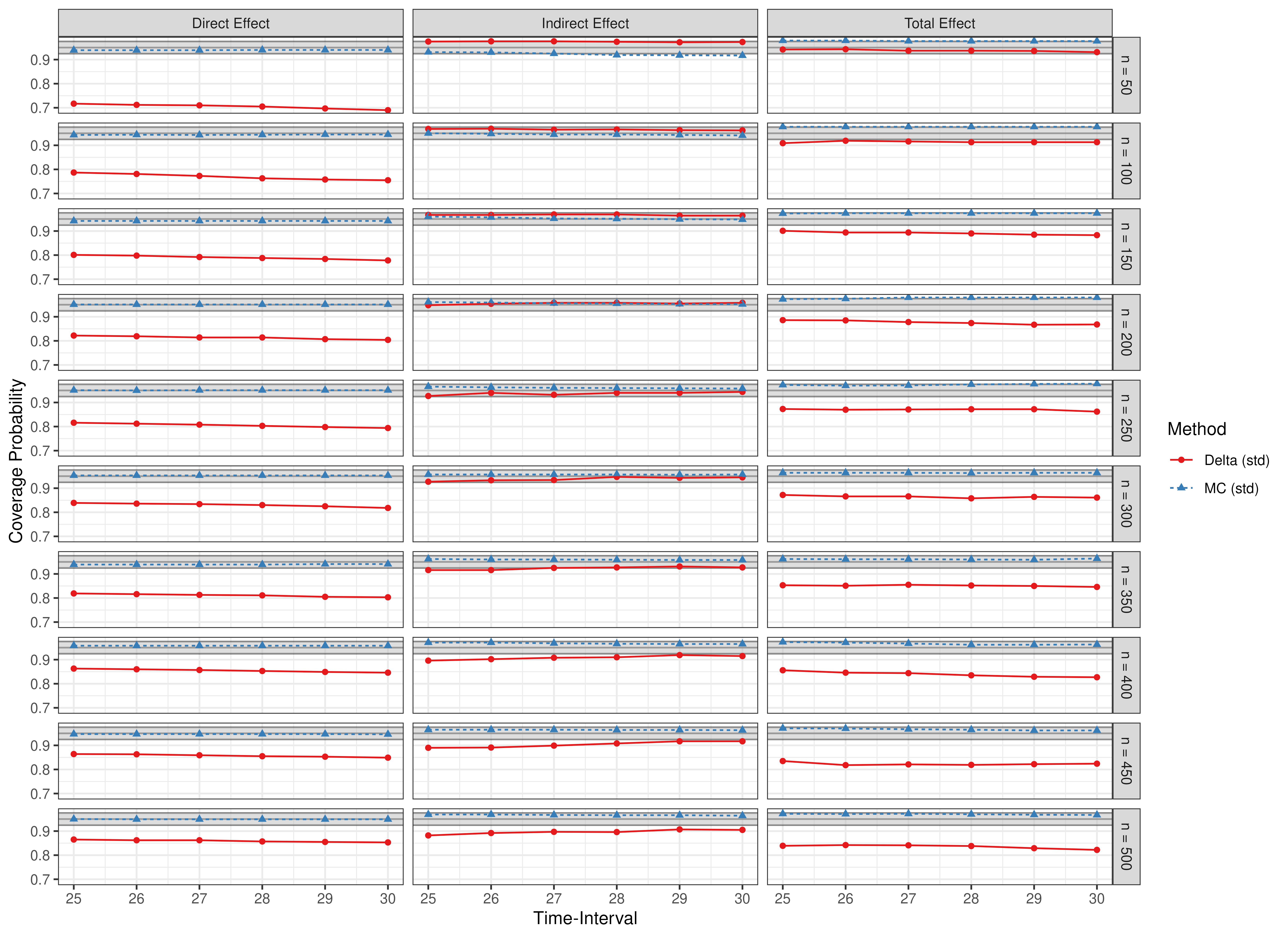
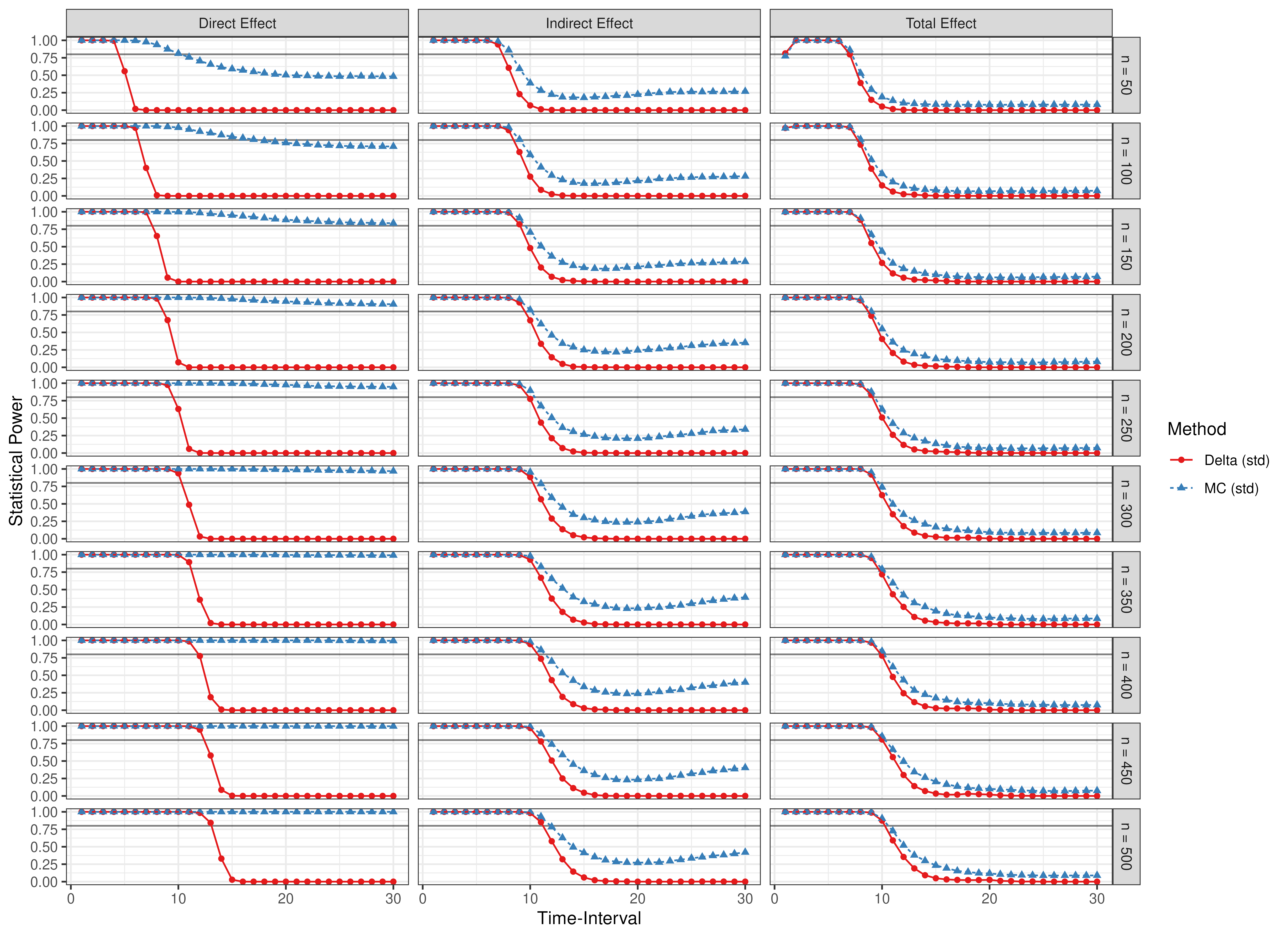
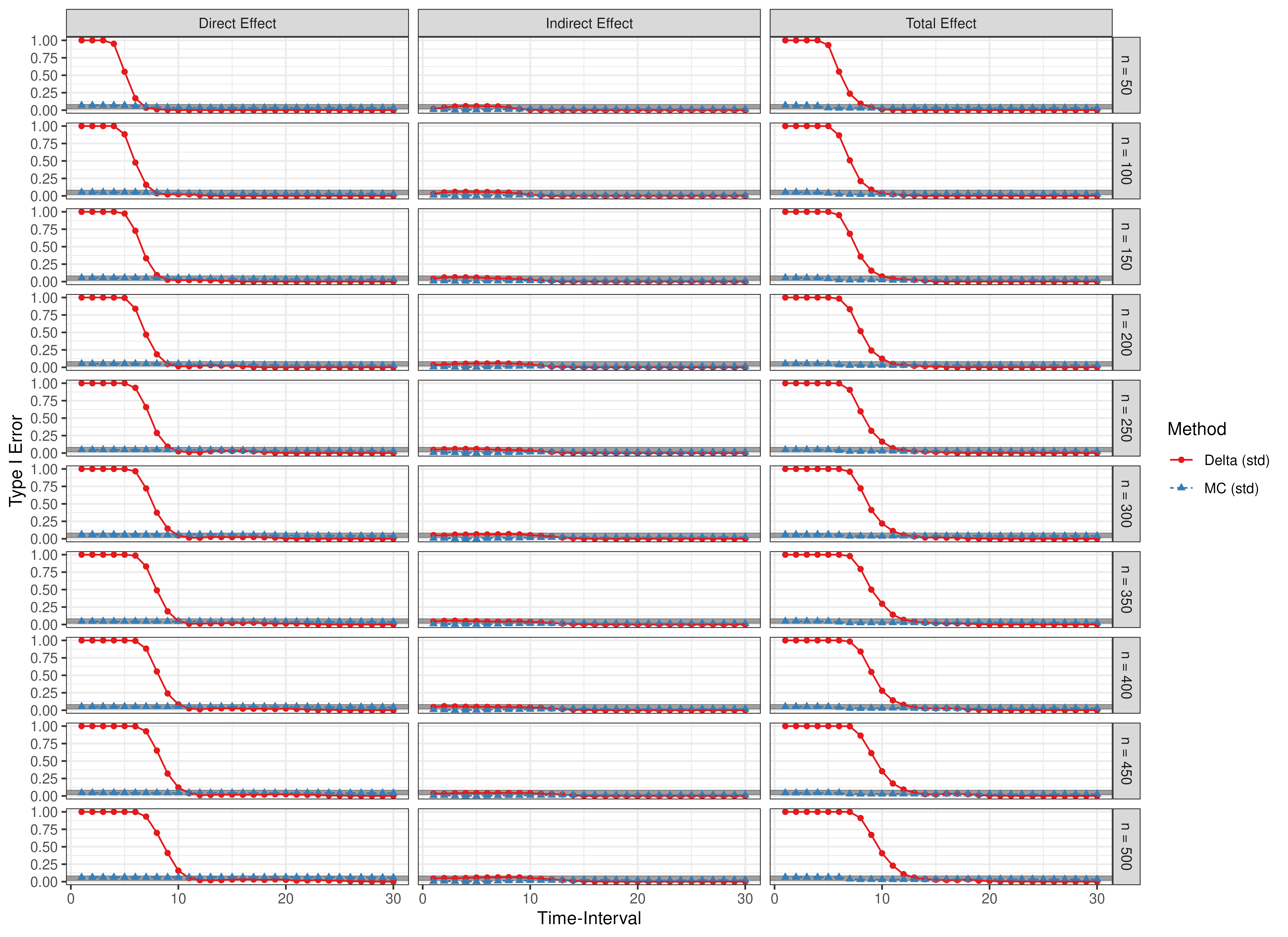
Evaluation of Confidence Intervals

Presented below are scatter plots of coverage probabilities and power for the $\eta_X \to \eta_M \ to \eta_Y$ model and type I error rates for the $\eta_Y \to \eta_M \to \eta_X$ model.

data(results, package = "manCTMed")

Coverage Probabilities

Time Intervals 1 to 25

Time Intervals 1 to 4

Time Intervals 5 to 25

Time Intervals 25 to 30

Statistical Power

Type I Error Rate

Coverage Probabilities (Standardized)

Time Intervals 1 to 25

Time Intervals 1 to 4

Time Intervals 5 to 25

Time Intervals 25 to 30

Statistical Power (Standardized)

Type I Error Rate (Standardized)