Scatter Plots - Illustration

Ivan Jacob Agaloos Pesigan

library(manCTMed)

Population Total, Direct, and Indirect Effects

Total, direct, and indirect effects for the drift matrix

$$\begin{equation} \left( \begin{array}{ccc} -0.138 & 0 & 0 \\ -0.124 & -0.865 & 0.434 \\ -0.057 & 0.115 & -0.693 \\ \end{array} \right) \end{equation}$$

IllustrationFigPlotEffects(std = FALSE)
#> 
#> phi:
#>        x      m      y
#> x -0.138  0.000  0.000
#> m -0.124 -0.865  0.434
#> y -0.057  0.115 -0.693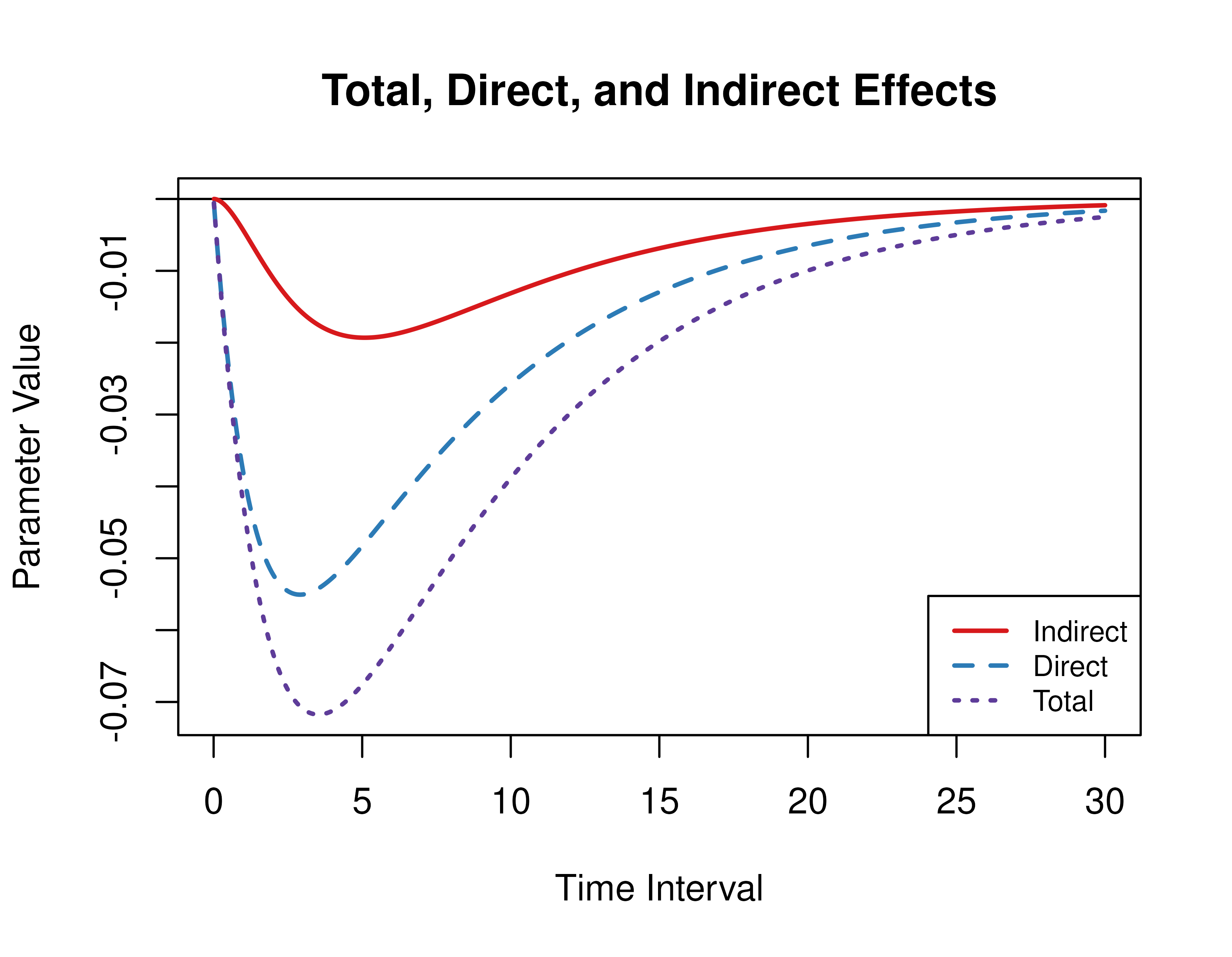

Standardized total, direct, and indirect effects for the drift matrix $$\begin{equation} \left( \begin{array}{ccc} -0.138 & 0 & 0 \\ -0.124 & -0.865 & 0.434 \\ -0.057 & 0.115 & -0.693 \\ \end{array} \right) \end{equation}$$ and process noise covariance matrix $$\begin{equation} \left( \begin{array}{ccc} 0.10 & 0 & 0 \\ 0 & 0.10 & 0 \\ 0 & 0 & 0.10 \\ \end{array} \right) \end{equation}$$

IllustrationFigPlotEffects(std = TRUE)
#> 
#> phi:
#>        x      m      y
#> x -0.138  0.000  0.000
#> m -0.124 -0.865  0.434
#> y -0.057  0.115 -0.693
#> 
#> sigma:
#>      [,1] [,2] [,3]
#> [1,]  0.1  0.0  0.0
#> [2,]  0.0  0.1  0.0
#> [3,]  0.0  0.0  0.1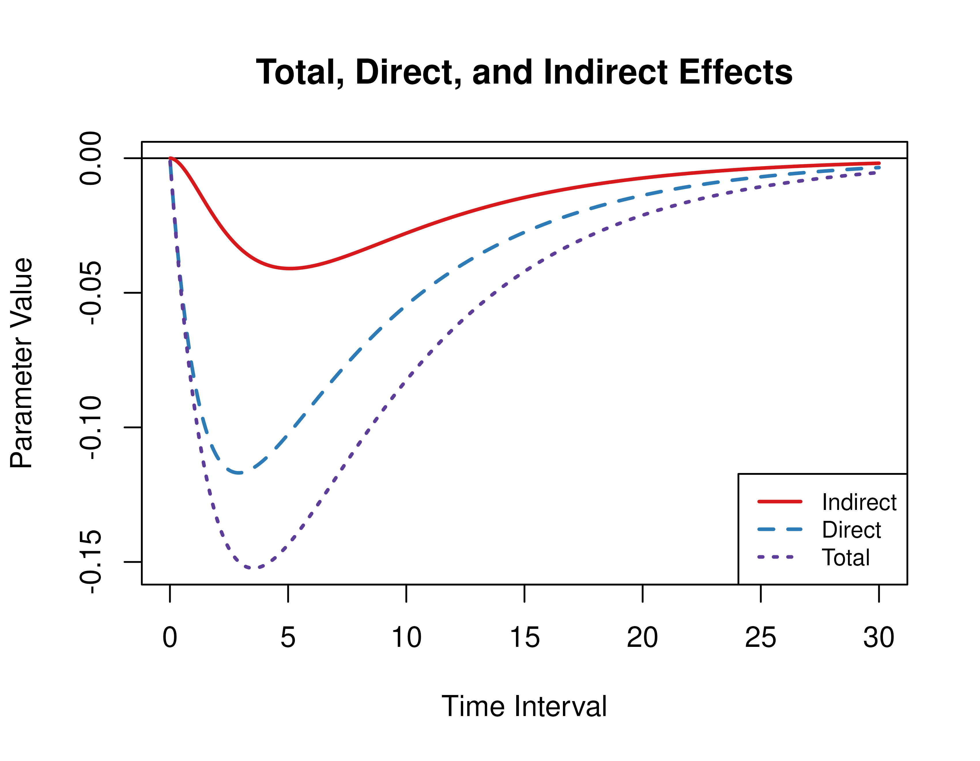

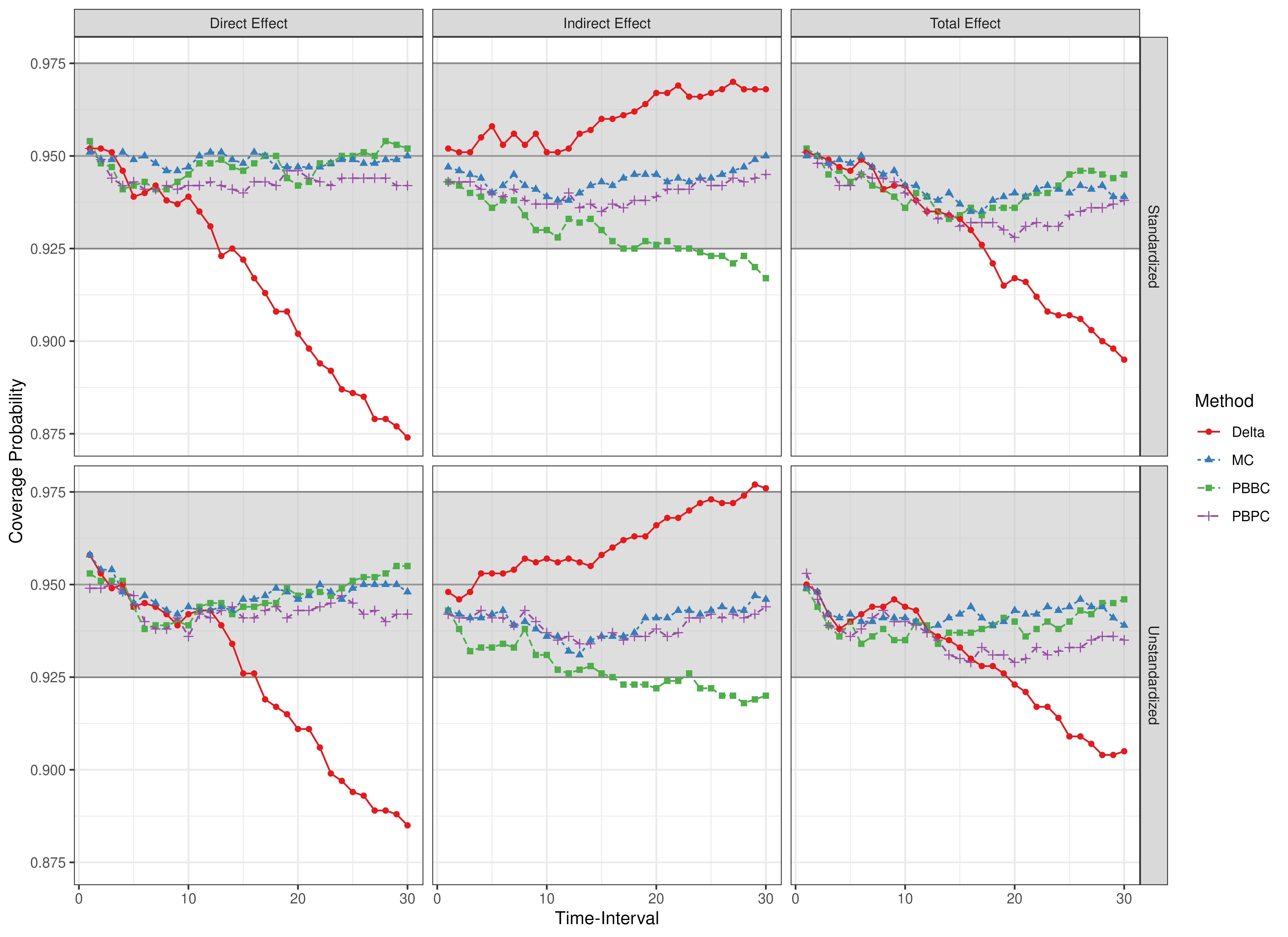
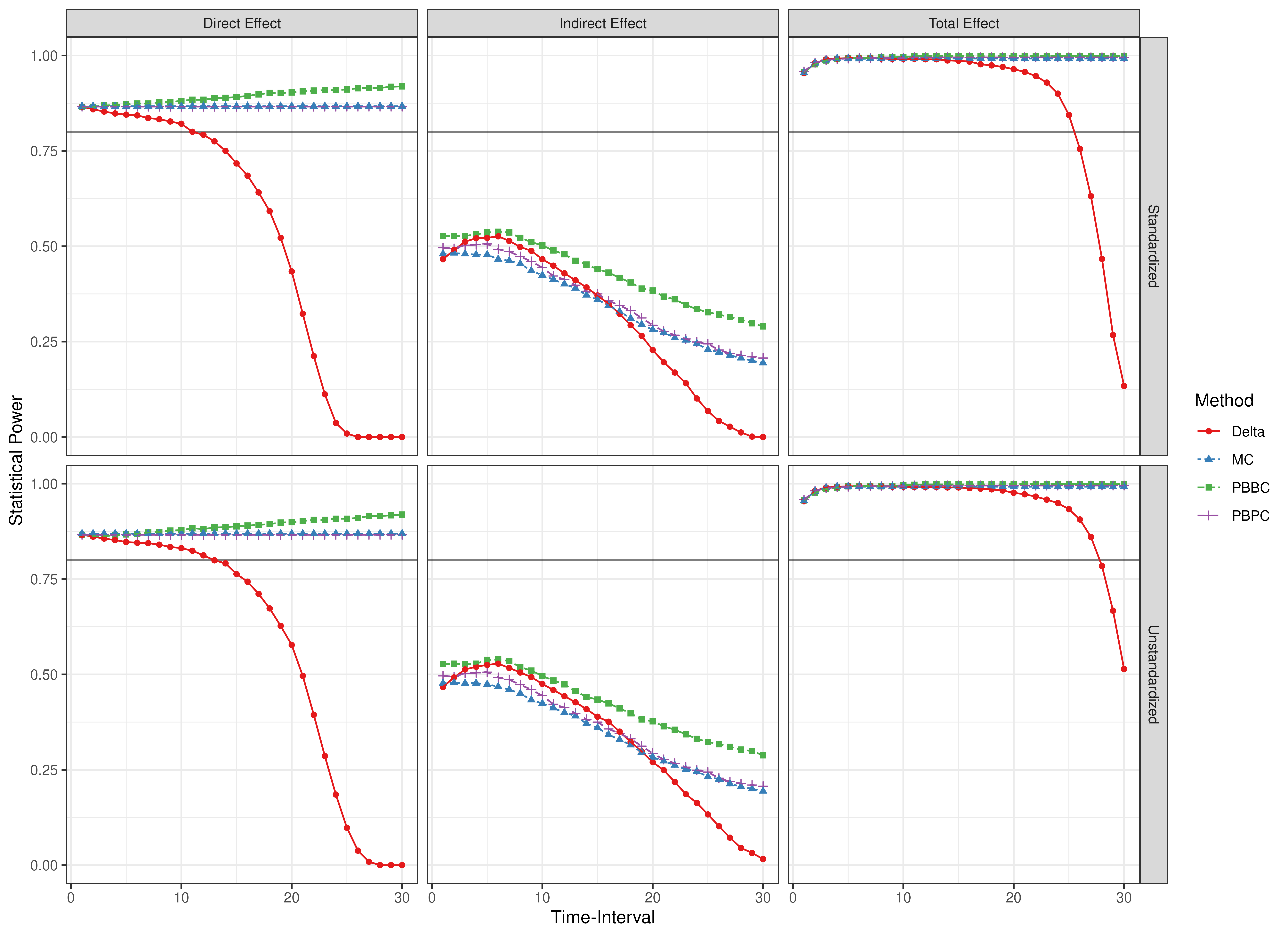
Evaluation of Confidence Intervals

Presented below are scatter plots of coverage probabilities and power for the $\eta_X \to \eta_M \ to \eta_Y$ model.

data(illustration_results, package = "manCTMed")

Coverage Probabilities

Statistical Power