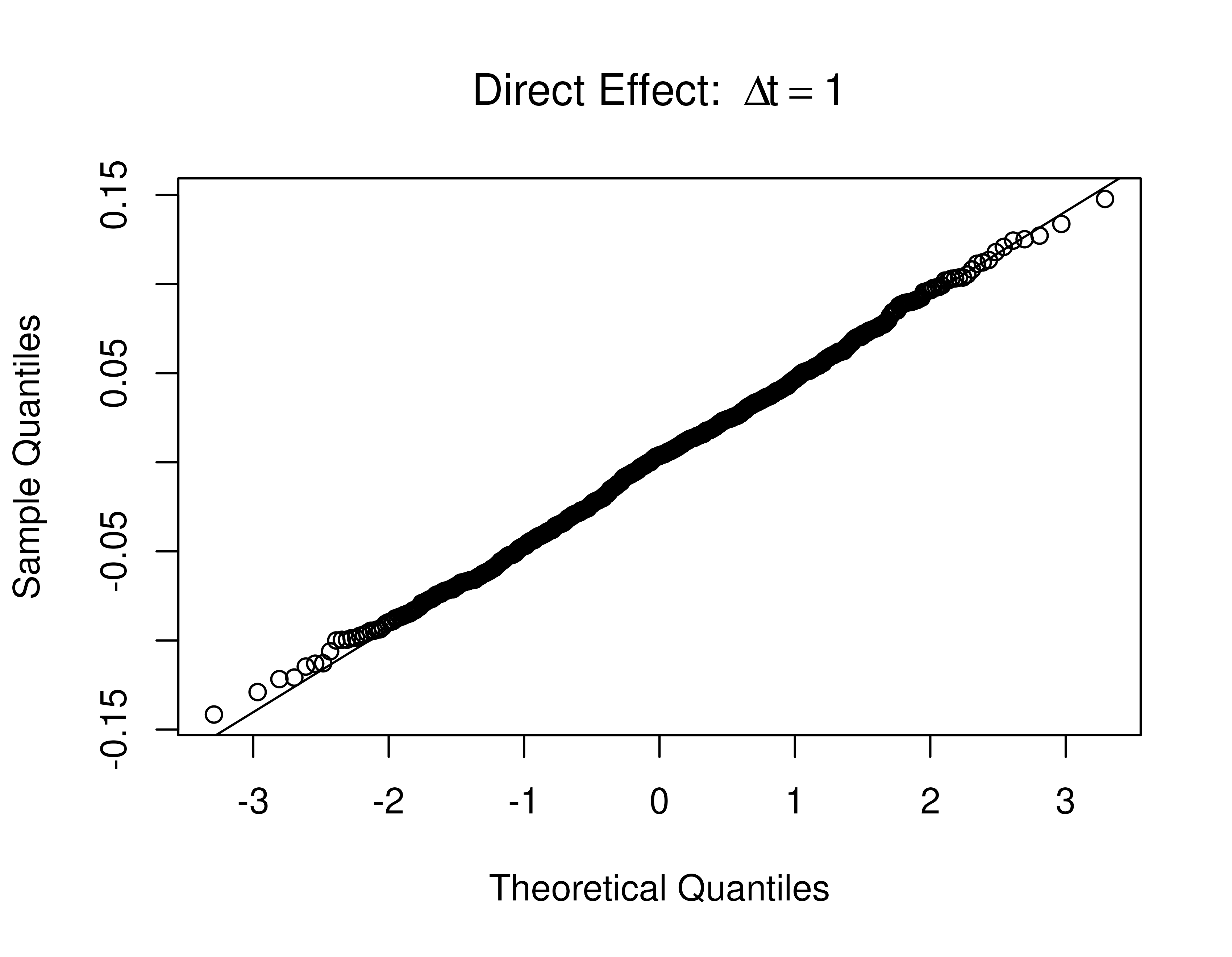
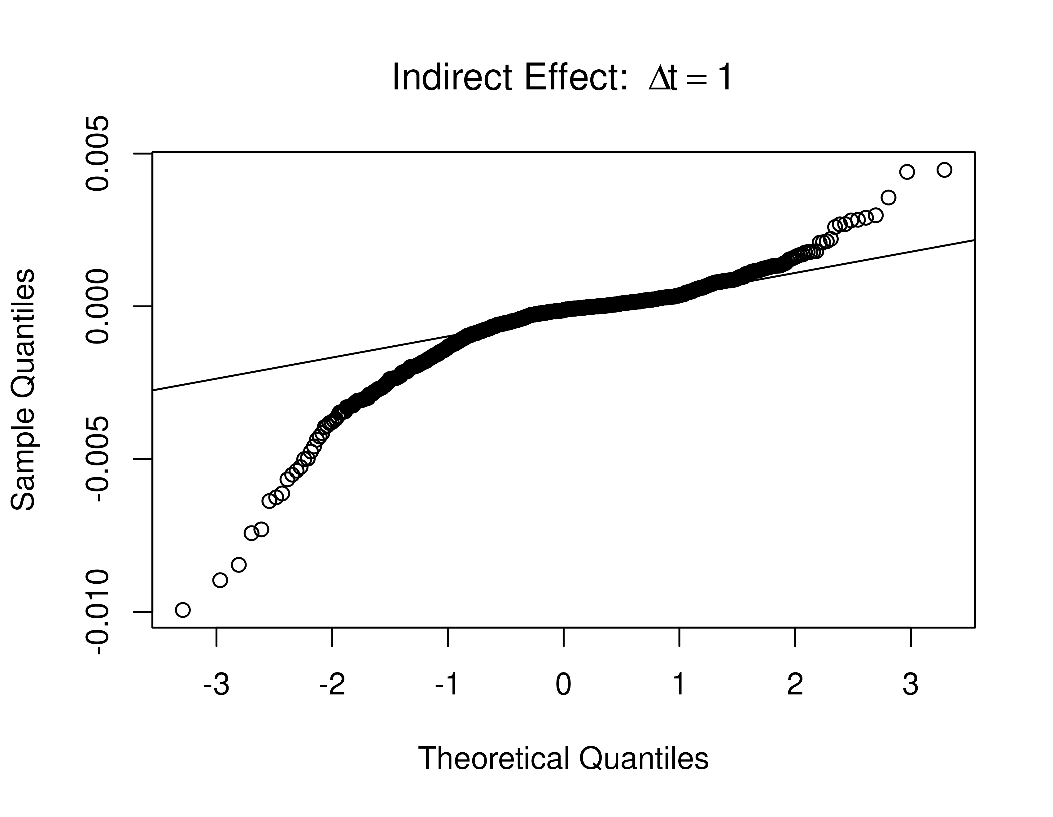
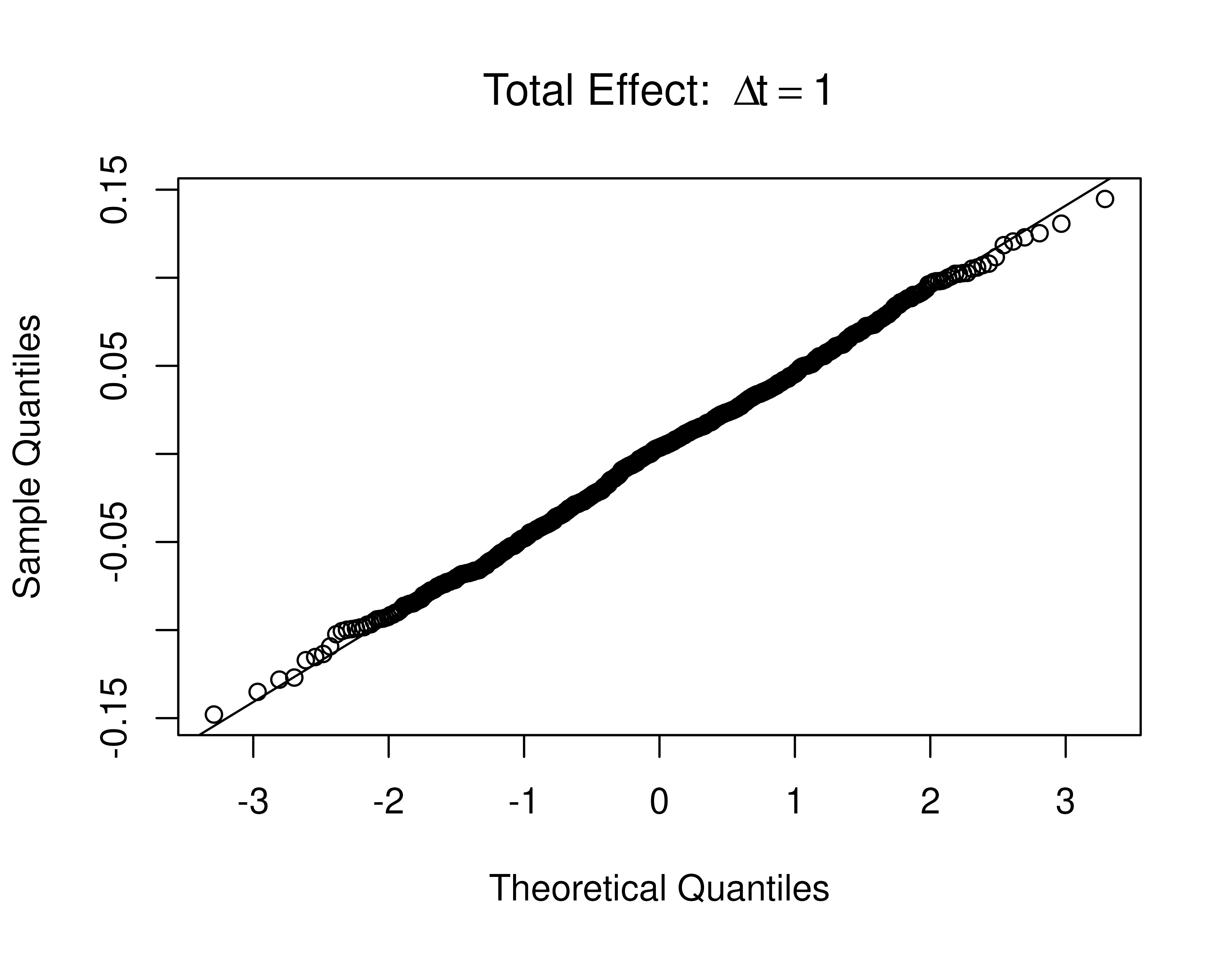
Skip to contents

Population Total, Direct, and Indirect Effects

Total, direct, and indirect effects for the drift matrix

(0.357000.7710.51100.4500.7290.693)\begin{equation} \left( \begin{array}{ccc} -0.357 & 0 & 0 \\ 0.771 & -0.511 & 0 \\ -0.450 & 0.729 & -0.693 \\ \end{array} \right) \end{equation}

Presented below are the effects for the ηYηMηX\eta_{Y} \to \eta_{M} \to \eta_{X} model.

FigPlotEffects(dynamics = 0, xmy = FALSE)
#> 
#> phi:
#>        x      m      y
#> x -0.357  0.000  0.000
#> m  0.771 -0.511  0.000
#> y -0.450  0.729 -0.693

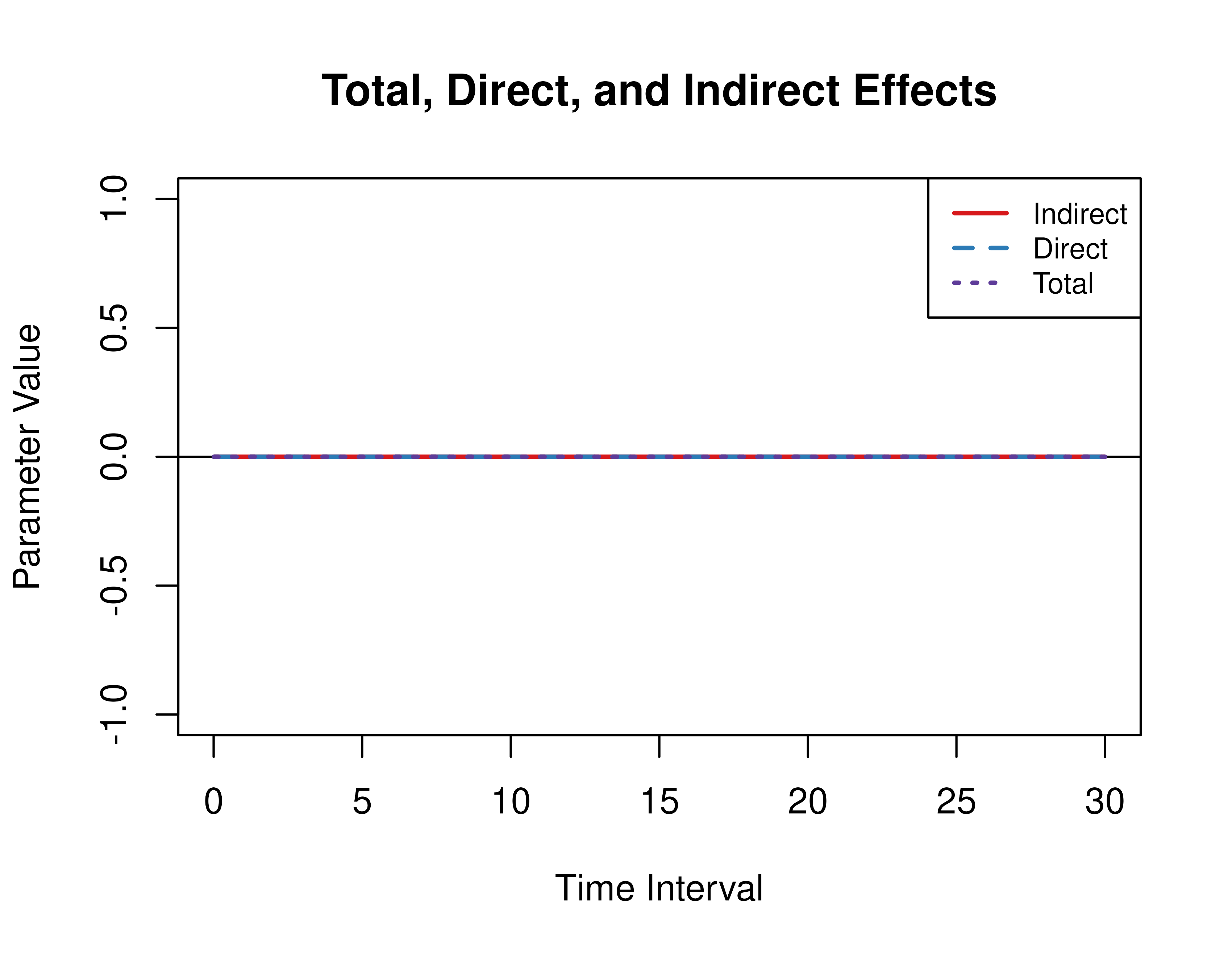
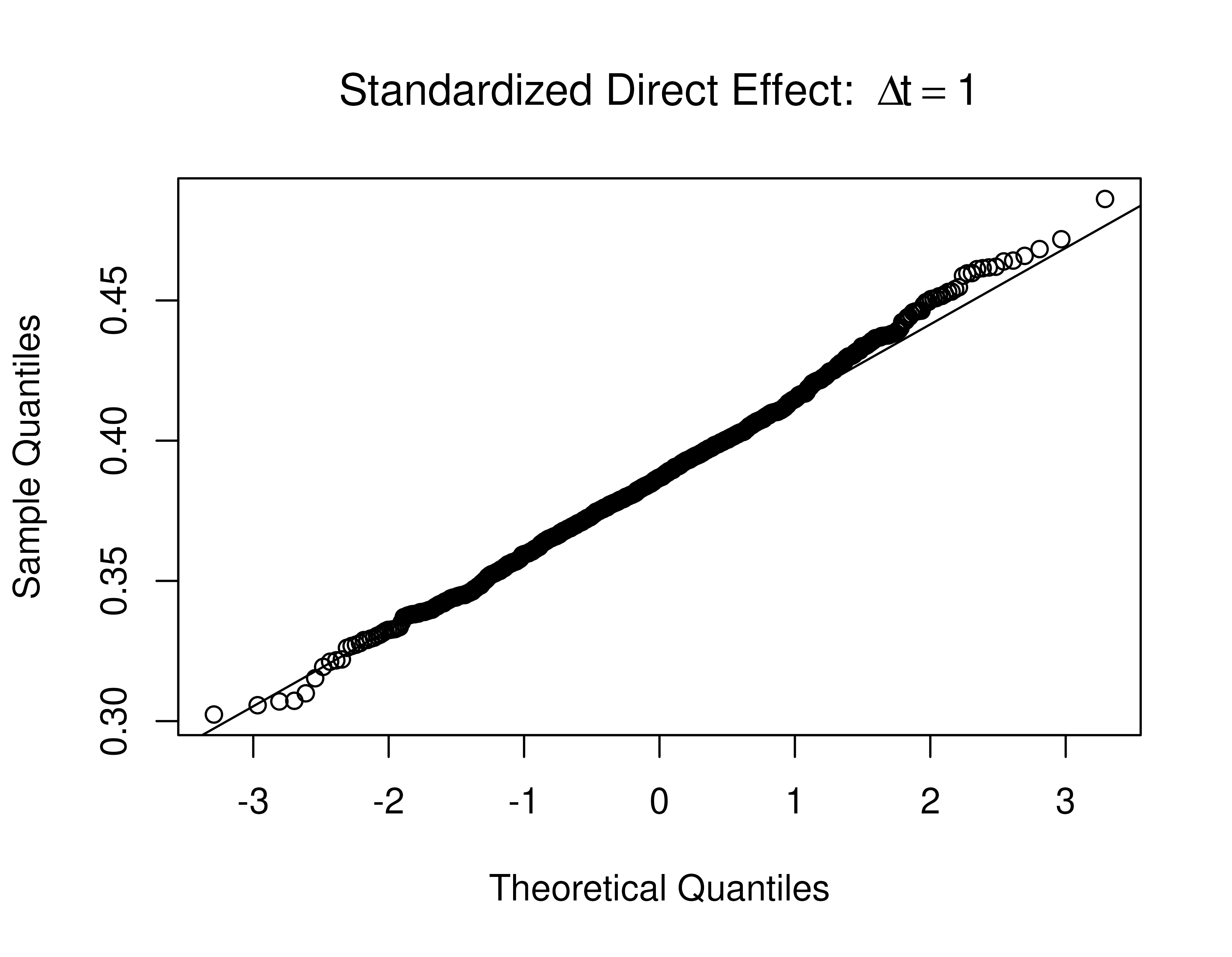
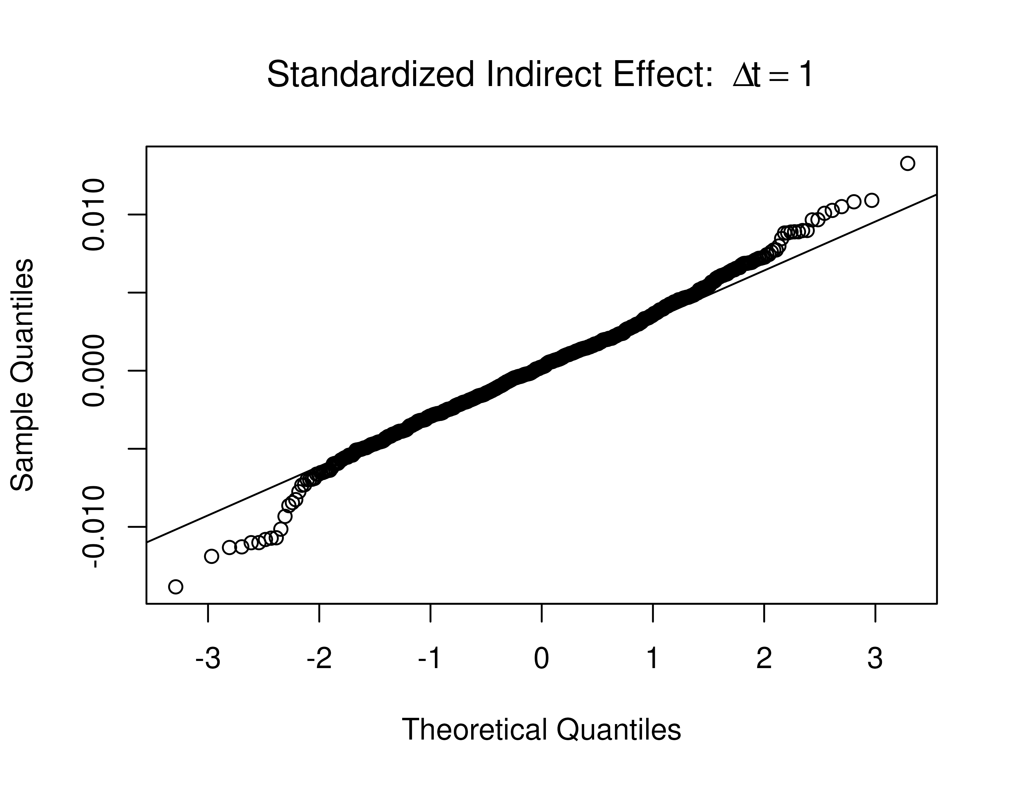
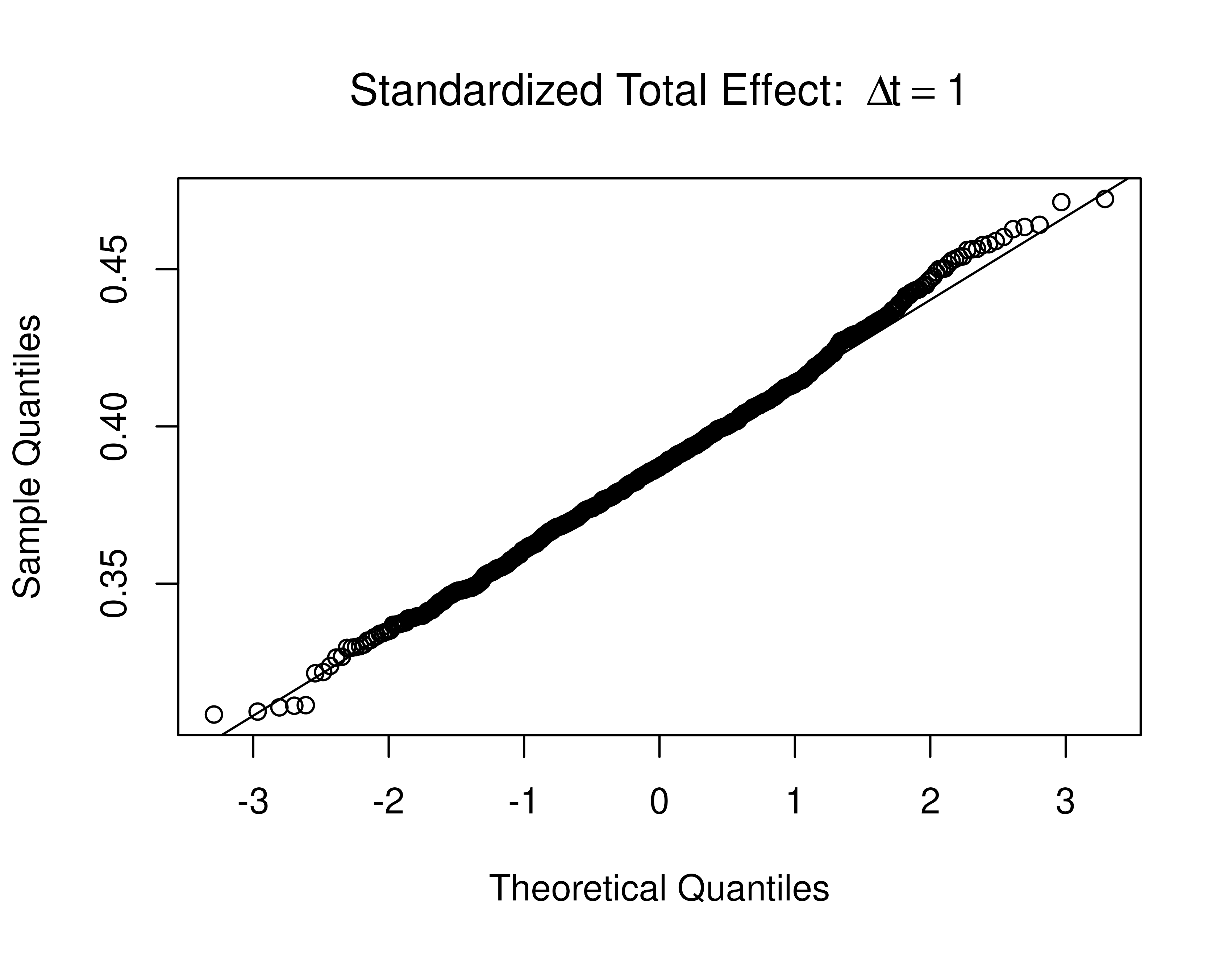
Standardized total, direct, and indirect effects for the drift matrix (0.357000.7710.51100.4500.7290.693)\begin{equation} \left( \begin{array}{ccc} -0.357 & 0 & 0 \\ 0.771 & -0.511 & 0 \\ -0.450 & 0.729 & -0.693 \\ \end{array} \right) \end{equation} and process noise covariance matrix (0.244555560.022015870.050047620.022015870.070678000.015394560.050047620.015394560.07553061)\begin{equation} \left( \begin{array}{ccc} 0.24455556 & 0.02201587 & -0.05004762 \\ 0.02201587 & 0.07067800 & 0.01539456 \\ -0.05004762 & 0.01539456 & 0.07553061 \\ \end{array} \right) \end{equation}

Presented below are the standardized effects for the ηYηMηX\eta_{Y} \to \eta_{M} \to \eta_{X} model.

FigPlotEffects(dynamics = 0, std = TRUE, xmy = FALSE)
#> 
#> phi:
#>        x      m      y
#> x -0.357  0.000  0.000
#> m  0.771 -0.511  0.000
#> y -0.450  0.729 -0.693
#> 
#> sigma:
#>             [,1]       [,2]        [,3]
#> [1,]  0.24455556 0.02201587 -0.05004762
#> [2,]  0.02201587 0.07067800  0.01539456
#> [3,] -0.05004762 0.01539456  0.07553061

Visualizing Normality of the Direct, Indirect, and Total Effects

The sampling distribution of the direct, indirect, and total effects were generated using 1000 samples.

Visualizing Normality of the Standardized Direct, Indirect, and Total Effects

The sampling distribution of the standardized direct, indirect, and total effects were generated using 1000 samples.