The Vector Autoregressive Model

Ivan Jacob Agaloos Pesigan

2025-05-10

Model

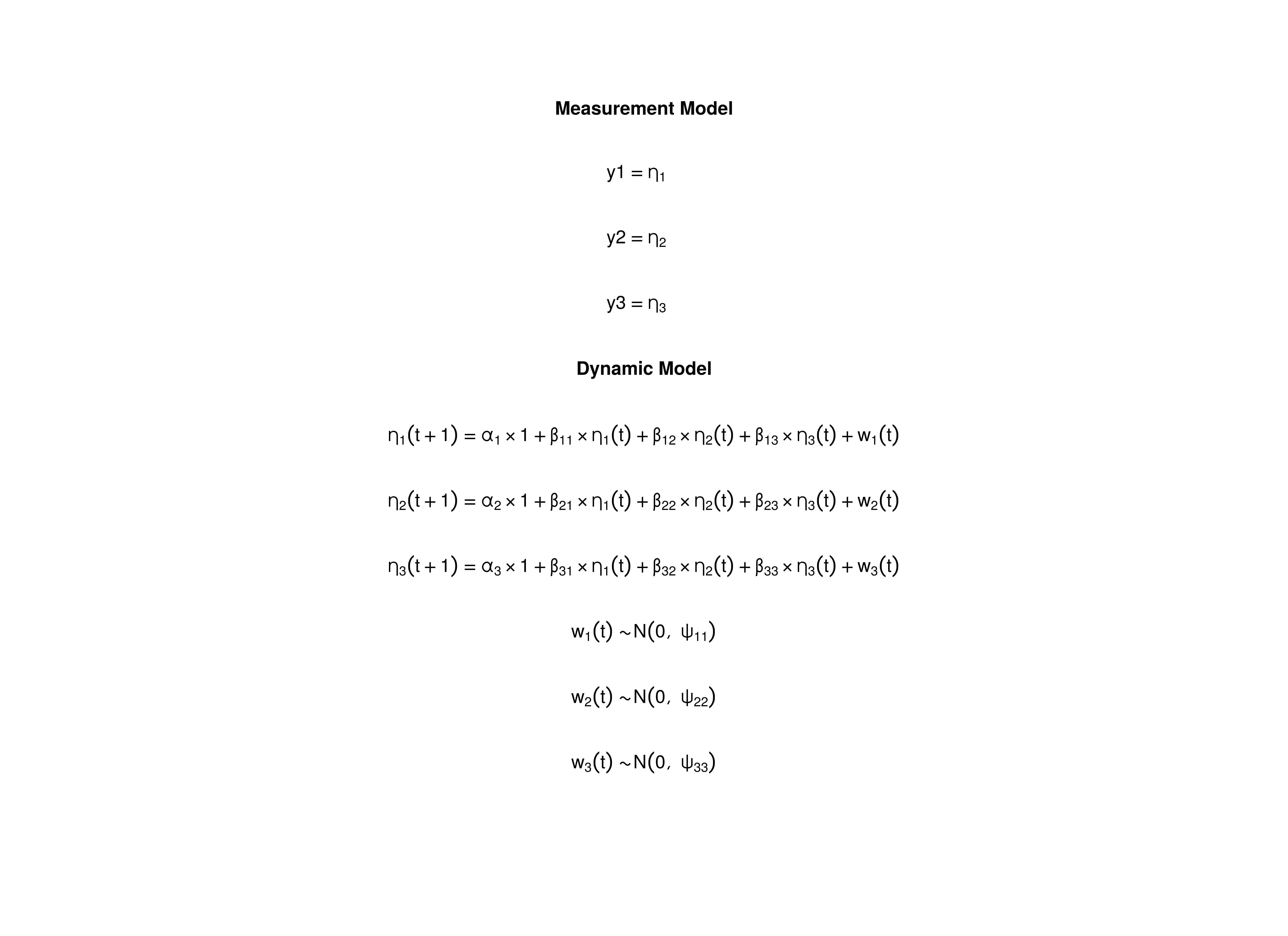
The measurement model is given by $$\begin{equation} \mathbf{y}_{i, t} = \boldsymbol{\eta}_{i, t} \end{equation}$$ where $\mathbf{y}_{i, t}$ represents a vector of observed variables and $\boldsymbol{\eta}_{i, t}$ a vector of latent variables for individual $i$ and time $t$. Since the observed and latent variables are equal, we only generate data from the dynamic structure.

The dynamic structure is given by $$\begin{equation} \boldsymbol{\eta}_{i, t} = \boldsymbol{\alpha} + \boldsymbol{\beta} \boldsymbol{\eta}_{i, t - 1} + \boldsymbol{\zeta}_{i, t}, \quad \mathrm{with} \quad \boldsymbol{\zeta}_{i, t} \sim \mathcal{N} \left( \mathbf{0}, \boldsymbol{\Psi} \right) \end{equation}$$ where $\boldsymbol{\eta}_{i, t}$, $\boldsymbol{\eta}_{i, t - 1}$, and $\boldsymbol{\zeta}_{i, t}$ are random variables, and $\boldsymbol{\alpha}$, $\boldsymbol{\beta}$, and $\boldsymbol{\Psi}$ are model parameters. Here, $\boldsymbol{\eta}_{i, t}$ is a vector of latent variables at time $t$ and individual $i$, $\boldsymbol{\eta}_{i, t - 1}$ represents a vector of latent variables at time $t - 1$ and individual $i$, and $\boldsymbol{\zeta}_{i, t}$ represents a vector of dynamic noise at time $t$ and individual $i$. $\boldsymbol{\alpha}$ denotes a vector of intercepts, $\boldsymbol{\beta}$ a matrix of autoregression and cross regression coefficients, and $\boldsymbol{\Psi}$ the covariance matrix of $\boldsymbol{\zeta}_{i, t}$.

An alternative representation of the dynamic noise is given by $$\begin{equation} \boldsymbol{\zeta}_{i, t} = \boldsymbol{\Psi}^{\frac{1}{2}} \mathbf{z}_{i, t}, \quad \mathrm{with} \quad \mathbf{z}_{i, t} \sim \mathcal{N} \left( \mathbf{0}, \mathbf{I} \right) \end{equation}$$ where $\left( \boldsymbol{\Psi}^{\frac{1}{2}} \right) \left( \boldsymbol{\Psi}^{\frac{1}{2}} \right)^{\prime} = \boldsymbol{\Psi}$ .

Data Generation

Notation

Let $t = 1000$ be the number of time points and $n = 1000$ be the number of individuals.

Let the initial condition $\boldsymbol{\eta}_{0}$ be given by

$$\begin{equation} \boldsymbol{\eta}_{0} \sim \mathcal{N} \left( \boldsymbol{\mu}_{\boldsymbol{\eta} \mid 0}, \boldsymbol{\Sigma}_{\boldsymbol{\eta} \mid 0} \right) \end{equation}$$

$$\begin{equation} \boldsymbol{\mu}_{\boldsymbol{\eta} \mid 0} = \left( \begin{array}{c} 0 \\ 0 \\ 0 \\ \end{array} \right) \end{equation}$$

$$\begin{equation} \boldsymbol{\Sigma}_{\boldsymbol{\eta} \mid 0} = \left( \begin{array}{ccc} 0.1960784 & 0.1183232 & 0.0298539 \\ 0.1183232 & 0.3437711 & 0.1381855 \\ 0.0298539 & 0.1381855 & 0.2663828 \\ \end{array} \right) . \end{equation}$$

Let the constant vector $\boldsymbol{\alpha}$ be given by

$$\begin{equation} \boldsymbol{\alpha} = \left( \begin{array}{c} 0 \\ 0 \\ 0 \\ \end{array} \right) . \end{equation}$$

Let the transition matrix $\boldsymbol{\beta}$ be given by

$$\begin{equation} \boldsymbol{\beta} = \left( \begin{array}{ccc} 0.7 & 0 & 0 \\ 0.5 & 0.6 & 0 \\ -0.1 & 0.4 & 0.5 \\ \end{array} \right) . \end{equation}$$

Let the dynamic process noise $\boldsymbol{\Psi}$ be given by

$$\begin{equation} \boldsymbol{\Psi} = \left( \begin{array}{ccc} 0.1 & 0 & 0 \\ 0 & 0.1 & 0 \\ 0 & 0 & 0.1 \\ \end{array} \right) . \end{equation}$$

R Function Arguments

n
#> [1] 1000
time
#> [1] 1000
mu0
#> [1] 0 0 0
sigma0
#>            [,1]      [,2]       [,3]
#> [1,] 0.19607843 0.1183232 0.02985385
#> [2,] 0.11832319 0.3437711 0.13818551
#> [3,] 0.02985385 0.1381855 0.26638284
sigma0_l # sigma0_l <- t(chol(sigma0))
#>            [,1]      [,2]     [,3]
#> [1,] 0.44280744 0.0000000 0.000000
#> [2,] 0.26721139 0.5218900 0.000000
#> [3,] 0.06741949 0.2302597 0.456966
alpha
#> [1] 0 0 0
beta
#>      [,1] [,2] [,3]
#> [1,]  0.7  0.0  0.0
#> [2,]  0.5  0.6  0.0
#> [3,] -0.1  0.4  0.5
psi
#>      [,1] [,2] [,3]
#> [1,]  0.1  0.0  0.0
#> [2,]  0.0  0.1  0.0
#> [3,]  0.0  0.0  0.1
psi_l # psi_l <- t(chol(psi))
#>           [,1]      [,2]      [,3]
#> [1,] 0.3162278 0.0000000 0.0000000
#> [2,] 0.0000000 0.3162278 0.0000000
#> [3,] 0.0000000 0.0000000 0.3162278

Visualizing the Dynamics Without Process Noise (n = 5 with Different Initial Condition)

Using the SimSSMVARFixed Function from the simStateSpace Package to Simulate Data

library(simStateSpace)
sim <- SimSSMVARFixed(
  n = n,
  time = time,
  mu0 = mu0,
  sigma0_l = sigma0_l,
  alpha = alpha,
  beta = beta,
  psi_l = psi_l
)
data <- as.data.frame(sim)
head(data)
#>   id time          y1          y2          y3
#> 1  1    0 -0.81728749  0.01319023  0.57975035
#> 2  1    1 -0.62264147 -0.94877859  0.54422379
#> 3  1    2 -0.06731464 -0.69530903 -0.09626706
#> 4  1    3 -0.09174342 -0.44804477 -0.27983813
#> 5  1    4 -0.04104160 -0.72769549 -0.19238403
#> 6  1    5  0.18907246 -0.81602072 -0.73831208
summary(data)
#>        id              time             y1                   y2            
#>  Min.   :   1.0   Min.   :  0.0   Min.   :-2.6043472   Min.   :-2.6896682  
#>  1st Qu.: 250.8   1st Qu.:249.8   1st Qu.:-0.2985133   1st Qu.:-0.3937008  
#>  Median : 500.5   Median :499.5   Median :-0.0006372   Median :-0.0001104  
#>  Mean   : 500.5   Mean   :499.5   Mean   :-0.0003479   Mean   : 0.0002634  
#>  3rd Qu.: 750.2   3rd Qu.:749.2   3rd Qu.: 0.2976899   3rd Qu.: 0.3954906  
#>  Max.   :1000.0   Max.   :999.0   Max.   : 2.1090871   Max.   : 2.8792429  
#>        y3            
#>  Min.   :-2.4120953  
#>  1st Qu.:-0.3471103  
#>  Median :-0.0001755  
#>  Mean   :-0.0002761  
#>  3rd Qu.: 0.3470153  
#>  Max.   : 2.5320530
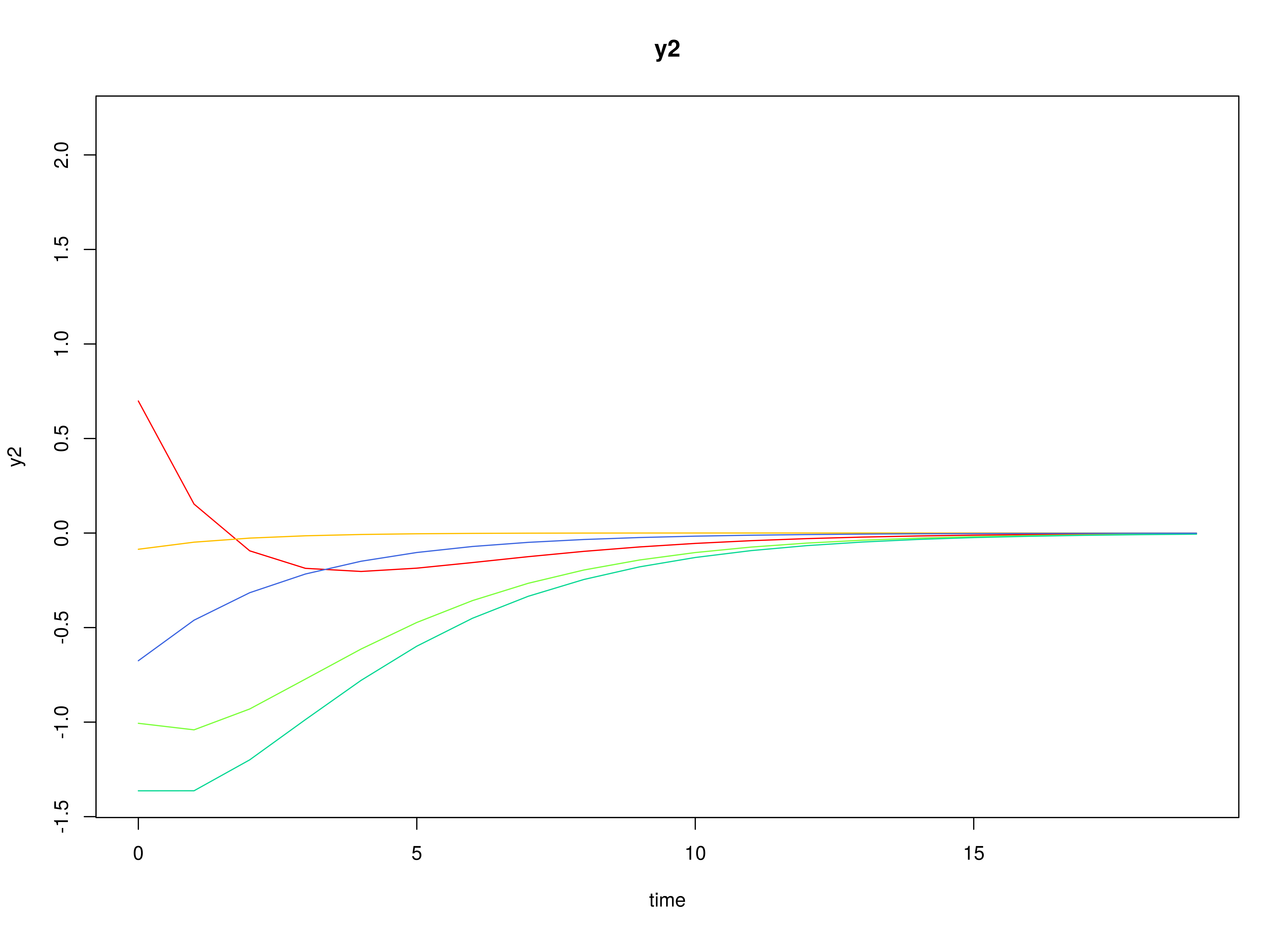
plot(sim)

Model Fitting

Prepare Data

dynr_data <- dynr::dynr.data(
  data = data,
  id = "id",
  time = "time",
  observed = c("y1", "y2", "y3")
)

Prepare Initial Condition

dynr_initial <- dynr::prep.initial(
  values.inistate = mu0,
  params.inistate = c("mu0_1_1", "mu0_2_1", "mu0_3_1"),
  values.inicov = sigma0,
  params.inicov = matrix(
    data = c(
      "sigma0_1_1", "sigma0_2_1", "sigma0_3_1",
      "sigma0_2_1", "sigma0_2_2", "sigma0_3_2",
      "sigma0_3_1", "sigma0_3_2", "sigma0_3_3"
    ),
    nrow = 3
  )
)

Prepare Measurement Model

dynr_measurement <- dynr::prep.measurement(
  values.load = diag(3),
  params.load = matrix(data = "fixed", nrow = 3, ncol = 3),
  state.names = c("eta_1", "eta_2", "eta_3"),
  obs.names = c("y1", "y2", "y3")
)

Prepare Dynamic Process

dynr_dynamics <- dynr::prep.formulaDynamics(
  formula = list(
    eta_1 ~ alpha_1_1 * 1 + beta_1_1 * eta_1 + beta_1_2 * eta_2 + beta_1_3 * eta_3,
    eta_2 ~ alpha_2_1 * 1 + beta_2_1 * eta_1 + beta_2_2 * eta_2 + beta_2_3 * eta_3,
    eta_3 ~ alpha_3_1 * 1 + beta_3_1 * eta_1 + beta_3_2 * eta_2 + beta_3_3 * eta_3
  ),
  startval = c(
    alpha_1_1 = alpha[1], alpha_2_1 = alpha[2], alpha_3_1 = alpha[3],
    beta_1_1 = beta[1, 1], beta_1_2 = beta[1, 2], beta_1_3 = beta[1, 3],
    beta_2_1 = beta[2, 1], beta_2_2 = beta[2, 2], beta_2_3 = beta[2, 3],
    beta_3_1 = beta[3, 1], beta_3_2 = beta[3, 2], beta_3_3 = beta[3, 3]
  ),
  isContinuousTime = FALSE
)

Prepare Process Noise

dynr_noise <- dynr::prep.noise(
  values.latent = psi,
  params.latent = matrix(
    data = c(
      "psi_1_1", "psi_2_1", "psi_3_1",
      "psi_2_1", "psi_2_2", "psi_3_2",
      "psi_3_1", "psi_3_2", "psi_3_3"
    ),
    nrow = 3
  ),
  values.observed = matrix(data = 0, nrow = 3, ncol = 3),
  params.observed = matrix(data = "fixed", nrow = 3, ncol = 3)
)

Prepare the Model

model <- dynr::dynr.model(
  data = dynr_data,
  initial = dynr_initial,
  measurement = dynr_measurement,
  dynamics = dynr_dynamics,
  noise = dynr_noise,
  outfile = "var.c"
)

Fit the Model

results <- dynr::dynr.cook(
  model,
  debug_flag = TRUE,
  verbose = FALSE
)
#> [1] "Get ready!!!!"
#> using C compiler: ‘gcc (Ubuntu 13.3.0-6ubuntu2~24.04) 13.3.0’
#> Optimization function called.
#> Starting Hessian calculation ...
#> Finished Hessian calculation.
#> Original exit flag:  3 
#> Modified exit flag:  3 
#> Optimization terminated successfully: ftol_rel or ftol_abs was reached. 
#> Original fitted parameters:  -0.0001394231 0.0002063081 -0.0003589877 0.6994004 
#> 0.0003966713 0.000244815 0.4988629 0.5997508 -0.000859385 -0.1020317 0.3997827 
#> 0.5003559 -2.304621 0.00113747 -0.001355358 -2.302905 -0.0003322207 -2.303592 
#> -0.02658042 0.00959209 0.02274173 -1.629246 0.6477301 0.1786098 -1.305423 
#> 0.5084412 -1.486772 
#> 
#> Transformed fitted parameters:  -0.0001394231 0.0002063081 -0.0003589877 
#> 0.6994004 0.0003966713 0.000244815 0.4988629 0.5997508 -0.000859385 -0.1020317 
#> 0.3997827 0.5003559 0.09979666 0.0001135157 -0.0001352603 0.09996816 
#> -3.336531e-05 0.09989952 -0.02658042 0.00959209 0.02274173 0.1960773 0.1270052 
#> 0.03502133 0.353323 0.1605014 0.3024284 
#> 
#> Doing end processing
#> Successful trial
#> Total Time: 13.25697 
#> Backend Time: 13.2568

Summary

summary(results)
#> Coefficients:
#>              Estimate Std. Error  t value   ci.lower   ci.upper Pr(>|t|)    
#> alpha_1_1  -1.394e-04  3.161e-04   -0.441 -7.589e-04  4.800e-04   0.3296    
#> alpha_2_1   2.063e-04  3.163e-04    0.652 -4.137e-04  8.263e-04   0.2571    
#> alpha_3_1  -3.590e-04  3.162e-04   -1.135 -9.788e-04  2.608e-04   0.1281    
#> beta_1_1    6.994e-01  8.071e-04  866.534  6.978e-01  7.010e-01   <2e-16 ***
#> beta_1_2    3.967e-04  6.787e-04    0.584 -9.336e-04  1.727e-03   0.2795    
#> beta_1_3    2.448e-04  6.921e-04    0.354 -1.112e-03  1.601e-03   0.3618    
#> beta_2_1    4.989e-01  8.077e-04  617.616  4.973e-01  5.004e-01   <2e-16 ***
#> beta_2_2    5.998e-01  6.794e-04  882.760  5.984e-01  6.011e-01   <2e-16 ***
#> beta_2_3   -8.594e-04  6.927e-04   -1.241 -2.217e-03  4.983e-04   0.1074    
#> beta_3_1   -1.020e-01  8.074e-04 -126.370 -1.036e-01 -1.004e-01   <2e-16 ***
#> beta_3_2    3.998e-01  6.792e-04  588.613  3.985e-01  4.011e-01   <2e-16 ***
#> beta_3_3    5.004e-01  6.927e-04  722.373  4.990e-01  5.017e-01   <2e-16 ***
#> psi_1_1     9.980e-02  1.412e-04  706.780  9.952e-02  1.001e-01   <2e-16 ***
#> psi_2_1     1.135e-04  9.991e-05    1.136 -8.231e-05  3.093e-04   0.1280    
#> psi_3_1    -1.353e-04  9.988e-05   -1.354 -3.310e-04  6.050e-05   0.0878 .  
#> psi_2_2     9.997e-02  1.414e-04  706.782  9.969e-02  1.002e-01   <2e-16 ***
#> psi_3_2    -3.337e-05  9.996e-05   -0.334 -2.293e-04  1.625e-04   0.3693    
#> psi_3_3     9.990e-02  1.413e-04  706.748  9.962e-02  1.002e-01   <2e-16 ***
#> mu0_1_1    -2.658e-02  1.399e-02   -1.901 -5.399e-02  8.298e-04   0.0287 *  
#> mu0_2_1     9.592e-03  1.876e-02    0.511 -2.719e-02  4.637e-02   0.3046    
#> mu0_3_1     2.274e-02  1.738e-02    1.309 -1.132e-02  5.680e-02   0.0953 .  
#> sigma0_1_1  1.961e-01  8.756e-03   22.395  1.789e-01  2.132e-01   <2e-16 ***
#> sigma0_2_1  1.270e-01  9.301e-03   13.655  1.088e-01  1.452e-01   <2e-16 ***
#> sigma0_3_1  3.502e-02  7.817e-03    4.480  1.970e-02  5.034e-02   <2e-16 ***
#> sigma0_2_2  3.533e-01  1.594e-02   22.166  3.221e-01  3.846e-01   <2e-16 ***
#> sigma0_3_2  1.605e-01  1.153e-02   13.920  1.379e-01  1.831e-01   <2e-16 ***
#> sigma0_3_3  3.024e-01  1.361e-02   22.219  2.758e-01  3.291e-01   <2e-16 ***
#> ---
#> Signif. codes:  0 '***' 0.001 '**' 0.01 '*' 0.05 '.' 0.1 ' ' 1
#> 
#> -2 log-likelihood value at convergence = 1605208.90
#> AIC = 1605262.90
#> BIC = 1605581.92

Parameter Estimates

alpha_hat
#> [1] -0.0001394231  0.0002063081 -0.0003589877
beta_hat
#>            [,1]         [,2]         [,3]
#> [1,]  0.6994004 0.0003966713  0.000244815
#> [2,]  0.4988629 0.5997507880 -0.000859385
#> [3,] -0.1020317 0.3997826709  0.500355859
psi_hat
#>               [,1]          [,2]          [,3]
#> [1,]  0.0997966649  1.135157e-04 -1.352603e-04
#> [2,]  0.0001135157  9.996816e-02 -3.336531e-05
#> [3,] -0.0001352603 -3.336531e-05  9.989952e-02
mu0_hat
#> [1] -0.02658042  0.00959209  0.02274173
sigma0_hat
#>            [,1]      [,2]       [,3]
#> [1,] 0.19607732 0.1270052 0.03502133
#> [2,] 0.12700518 0.3533230 0.16050136
#> [3,] 0.03502133 0.1605014 0.30242838

References

Chow, S.-M., Ho, M. R., Hamaker, E. L., & Dolan, C. V. (2010). Equivalence and differences between structural equation modeling and state-space modeling techniques. Structural Equation Modeling: A Multidisciplinary Journal, 17(2), 303–332. https://doi.org/10.1080/10705511003661553

Ou, L., Hunter, M. D., & Chow, S.-M. (2019). What’s for dynr: A package for linear and nonlinear dynamic modeling in R. The R Journal, 11(1), 91. https://doi.org/10.32614/rj-2019-012

R Core Team. (2024). R: A language and environment for statistical computing. R Foundation for Statistical Computing. https://www.R-project.org/