MCStd Function Use Case 4: Difference of Standardized Regression Coefficients in Multiple Groups
Ivan Jacob Agaloos Pesigan
2026-06-14
Source:vignettes/mcstd-4-difference-regression-coefficients-multigroup.Rmd
mcstd-4-difference-regression-coefficients-multigroup.RmdThe MCStd() function is used to generate Monte Carlo
confidence intervals for differences between standardized regression
coefficients in multiple groups.
Data
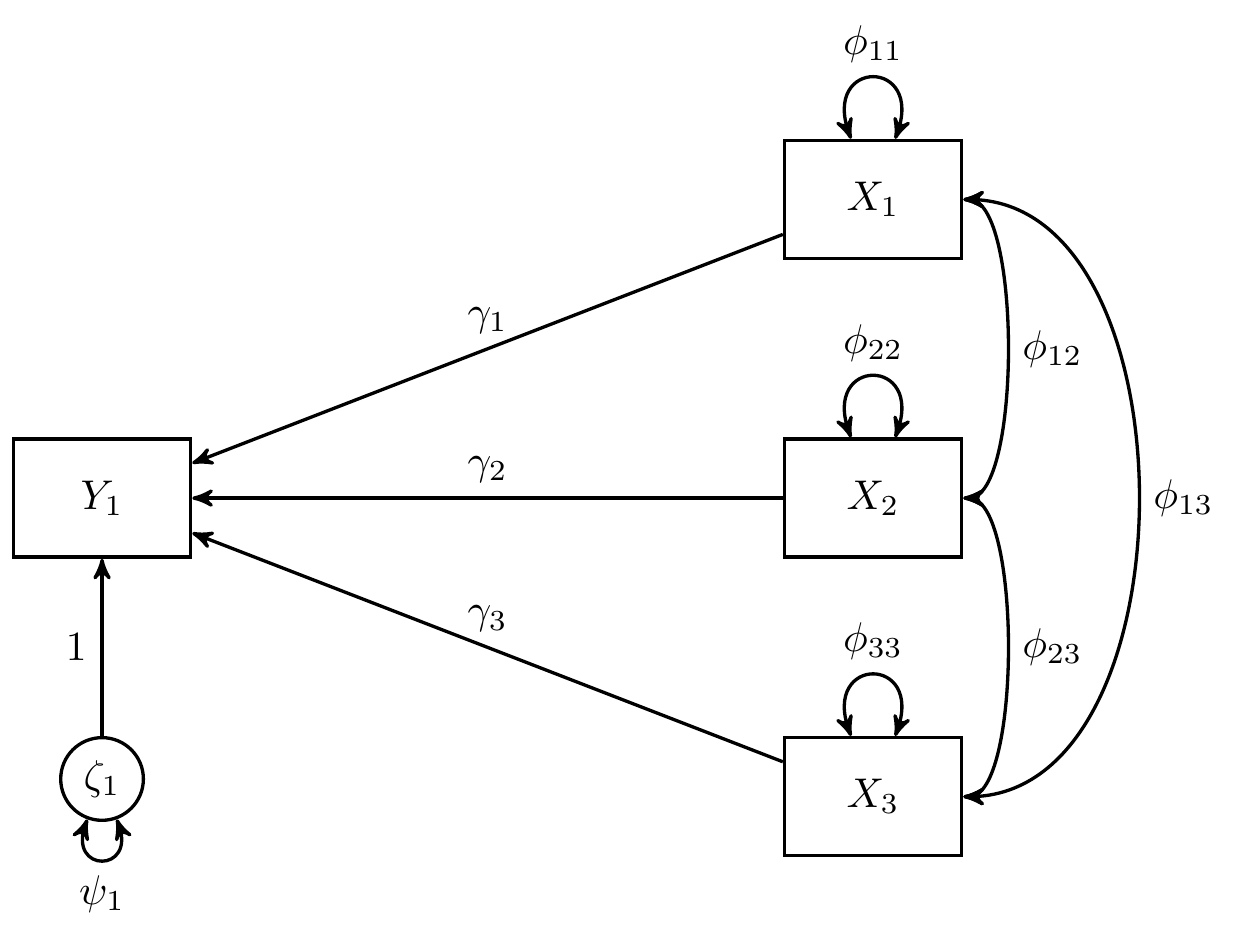
In this example, we use data from Kwan & Chan (2014) with three groups (Hong Kong, Japan, and Korea) where child’s reading ability () is regressed on parental occupational status (), parental educational level (), and child’s home possession ()
Note that is the stochastic error term with expected value of zero and finite variance , is the intercept, and , , and are regression coefficients.
knitr::kable(
  x = covs_hongkong, digits = 4,
  caption = "Covariance Matrix for Hong Kong"
)| Y1 | X1 | X2 | X3 | |
|---|---|---|---|---|
| Y1 | 8176.0021 | 27.3990 | 28.2320 | 31.2722 |
| X1 | 27.3990 | 0.9451 | 0.6006 | 0.4326 |
| X2 | 28.2320 | 0.6006 | 0.7977 | 0.3779 |
| X3 | 31.2722 | 0.4326 | 0.3779 | 0.8956 |
nobs_hongkong
#> [1] 4625
knitr::kable(
  x = covs_japan, digits = 4,
  caption = "Covariance Matrix for Japan"
)| Y1 | X1 | X2 | X3 | |
|---|---|---|---|---|
| Y1 | 9666.8658 | 34.2501 | 35.2189 | 30.6472 |
| X1 | 34.2501 | 1.0453 | 0.6926 | 0.5027 |
| X2 | 35.2189 | 0.6926 | 1.0777 | 0.4524 |
| X3 | 30.6472 | 0.5027 | 0.4524 | 0.9583 |
nobs_japan
#> [1] 5943
knitr::kable(
  x = covs_korea, digits = 4,
  caption = "Covariance Matrix for Korea"
)| Y1 | X1 | X2 | X3 | |
|---|---|---|---|---|
| Y1 | 8187.6921 | 31.6266 | 37.3062 | 30.9021 |
| X1 | 31.6266 | 0.9271 | 0.6338 | 0.4088 |
| X2 | 37.3062 | 0.6338 | 1.0007 | 0.3902 |
| X3 | 30.9021 | 0.4088 | 0.3902 | 0.8031 |
nobs_korea
#> [1] 5151
Model Specification
We regress Y1 on X1, X2, and
X3. We label the regression coefficient
for the three groups as gamma1.g1, gamma1.g2,
and gamma1.g3,
for the three groups as gamma2.g1, gamma2.g2,
and gamma2.g3, and
for the three groups as gamma3.g1, gamma3.g2,
and gamma3.g3.
model <- "
  Y1 ~ c(gamma1.g1, gamma1.g2, gamma1.g3) * X1
  Y1 ~ c(gamma2.g1, gamma2.g2, gamma2.g3) * X2
  Y1 ~ c(gamma3.g1, gamma3.g2, gamma3.g3) * X3
  gamma1.g12 := gamma1.g1 - gamma1.g2
  gamma1.g13 := gamma1.g1 - gamma1.g3
  gamma1.g23 := gamma1.g2 - gamma1.g3
  gamma2.g12 := gamma2.g1 - gamma2.g2
  gamma2.g13 := gamma2.g1 - gamma2.g3
  gamma2.g23 := gamma2.g2 - gamma2.g3
  gamma3.g12 := gamma3.g1 - gamma3.g2
  gamma3.g13 := gamma3.g1 - gamma3.g3
  gamma3.g23 := gamma3.g2 - gamma3.g3
"
Model Fitting
We can now fit the model using the sem() function from
lavaan with mimic = "eqs" to ensure
compatibility with results from Kwan & Chan
(2011).
Note: We recommend setting
fixed.x = FALSEwhen generating standardized estimates and confidence intervals to model the variances and covariances of the exogenous observed variables if they are assumed to be random. Iffixed.x = TRUE, which is the default setting inlavaan,MC()will fix the variances and the covariances of the exogenous observed variables to the sample values.
Standardized Monte Carlo Confidence Intervals
Standardized Monte Carlo Confidence intervals can be generated by
passing the result of the MC() function to the
MCStd() function.
unstd <- MC(fit, R = 20000L, alpha = 0.05)
MCStd(unstd, alpha = 0.05)
#> Standardized Monte Carlo Confidence Intervals
#>                est     se     R    2.5%   97.5%
#> gamma1.g1   0.0568 0.0191 20000  0.0194  0.0942
#> gamma2.g1   0.1985 0.0186 20000  0.1616  0.2353
#> gamma3.g1   0.2500 0.0150 20000  0.2208  0.2791
#> Y1~~Y1      0.8215 0.0103 20000  0.8004  0.8409
#> X1~~X1      1.0000 0.0000 20000  1.0000  1.0000
#> X1~~X2      0.6917 0.0076 20000  0.6766  0.7064
#> X1~~X3      0.4702 0.0115 20000  0.4474  0.4923
#> X2~~X2      1.0000 0.0000 20000  1.0000  1.0000
#> X2~~X3      0.4471 0.0117 20000  0.4237  0.4699
#> X3~~X3      1.0000 0.0000 20000  1.0000  1.0000
#> gamma1.g2   0.1390 0.0164 20000  0.1068  0.1711
#> gamma2.g2   0.1792 0.0158 20000  0.1480  0.2098
#> gamma3.g2   0.1688 0.0139 20000  0.1416  0.1961
#> Y1~~Y1.g2   0.8371 0.0088 20000  0.8196  0.8539
#> X1~~X1.g2   1.0000 0.0000 20000  1.0000  1.0000
#> X1~~X2.g2   0.6525 0.0074 20000  0.6380  0.6670
#> X1~~X3.g2   0.5023 0.0096 20000  0.4833  0.5208
#> X2~~X2.g2   1.0000 0.0000 20000  1.0000  1.0000
#> X2~~X3.g2   0.4452 0.0104 20000  0.4249  0.4651
#> X3~~X3.g2   1.0000 0.0000 20000  1.0000  1.0000
#> gamma1.g3   0.0863 0.0170 20000  0.0527  0.1193
#> gamma2.g3   0.2557 0.0164 20000  0.2236  0.2877
#> gamma3.g3   0.2289 0.0139 20000  0.2017  0.2563
#> Y1~~Y1.g3   0.7761 0.0103 20000  0.7556  0.7958
#> X1~~X1.g3   1.0000 0.0000 20000  1.0000  1.0000
#> X1~~X2.g3   0.6580 0.0079 20000  0.6425  0.6734
#> X1~~X3.g3   0.4738 0.0107 20000  0.4526  0.4945
#> X2~~X2.g3   1.0000 0.0000 20000  1.0000  1.0000
#> X2~~X3.g3   0.4353 0.0112 20000  0.4133  0.4570
#> X3~~X3.g3   1.0000 0.0000 20000  1.0000  1.0000
#> gamma1.g12 -0.0821 0.0251 20000 -0.1311 -0.0336
#> gamma1.g13 -0.0294 0.0257 20000 -0.0802  0.0208
#> gamma1.g23  0.0527 0.0236 20000  0.0070  0.0993
#> gamma2.g12  0.0193 0.0244 20000 -0.0286  0.0674
#> gamma2.g13 -0.0572 0.0248 20000 -0.1059 -0.0081
#> gamma2.g23 -0.0765 0.0228 20000 -0.1213 -0.0320
#> gamma3.g12  0.0811 0.0203 20000  0.0411  0.1209
#> gamma3.g13  0.0211 0.0204 20000 -0.0191  0.0613
#> gamma3.g23 -0.0601 0.0196 20000 -0.0988 -0.0217