MCStd Function Use Case 3: R-Squared and Adjusted R-Squared

The MCStd() function is used to generate Monte Carlo confidence intervals for $R^{2}$ and adjusted $R^{2}$ $\left( \bar{R}^{2}\right)$.

library(semmcci)
library(lavaan)

Data

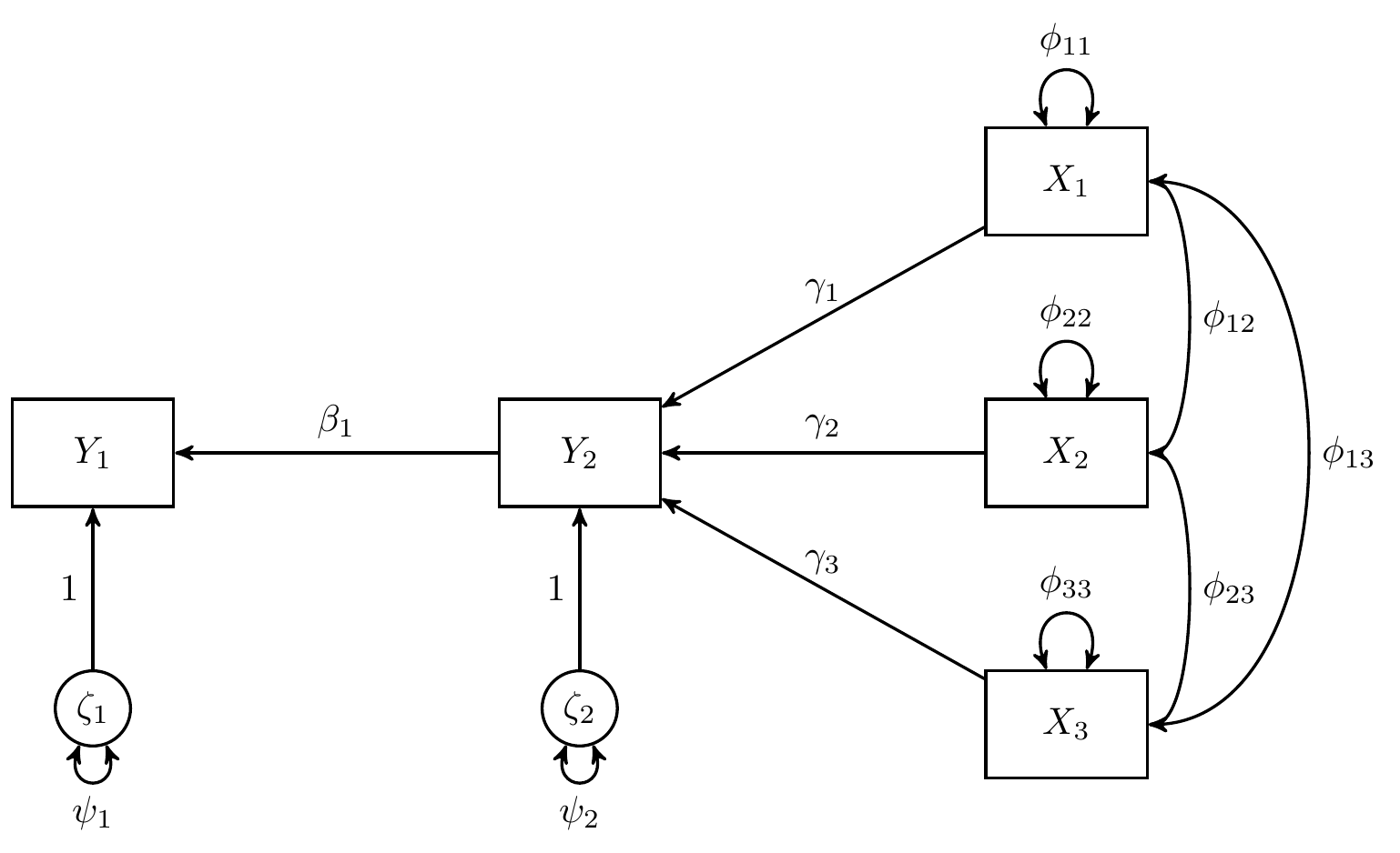
In this example, we use data from Kwan & Chan (2011) where child’s reading ability ($Y_{1}$) is regressed on home educational resources and home educational resources ($Y_{2}$) is regressed on parental occupational status ($X_{1}$), parental educational level ($X_{2}$), and child’s home possession ($X_{3}$)

\[ Y_{1} = \alpha_{1} + \beta_{1} Y_{2} + \zeta_{1} , \]

\[ Y_{2} = \alpha_{2} + \gamma_{1} X_{1} + \gamma_{2} X_{2} + \gamma_{3} X_{3} + \zeta_{2} . \]

Note that $\zeta_{1}$ and $\zeta_{2}$ are stochastic error terms with expected value of zero and finite variance $\psi_{1}$ and $\psi_{2}$, $\alpha_{1}$ and $\alpha_{2}$ are intercepts, and $\beta_{1}$, $\gamma_{1}$, $\gamma_{2}$, and $\gamma_{3}$ are regression coefficients.

$Mediation Model (Covariance Structure)$

Mediation Model (Covariance Structure)

covs
#>           Y1      Y2       X1      X2      X3
#> Y1 6088.8281 15.7012 271.1429 49.5848 20.0337
#> Y2   15.7012  0.7084   1.9878  1.0043  0.2993
#> X1  271.1429  1.9878 226.2577 29.9232  4.8812
#> X2   49.5848  1.0043  29.9232  9.0692  1.0312
#> X3   20.0337  0.2993   4.8812  1.0312  0.8371
nobs
#> [1] 200

Model Specification

We regress Y1 on Y2 and Y2 on X1, X2, and X3. We label the error variances as psi1 and psi2. $R^{2}$ and $\bar{R}^{2}$ are defined using the := operator in the lavaan model syntax using the following equations

\[ R^{2} = 1 - \psi^{\ast} \]

\[ \bar{R}^{2} = 1 - \left( \frac{n - 1}{n - p + 1} \right) \left( 1 - R^2 \right) \]

where $\psi^{\ast}$ is the standardized error variance, $n$ is the sample size, and $p$ is the number of regressor variables.

model <- "
  Y1 ~ Y2
  Y2 ~ X1 + X2 + X3
  Y1 ~~ psi1 * Y1
  Y2 ~~ psi2 * Y2
  rsq1 := 1 - psi1
  rsqbar1 := 1 - (
    (200 - 1) / (200 - 1 + 1)
  ) * (
    1 - rsq1
  )
  rsq2 := 1 - psi2
  rsqbar2 := 1 - (
    (200 - 1) / (200 - 3 + 1)
  ) * (
    1 - rsq2
  )
"

Model Fitting

We can now fit the model using the sem() function from lavaan with mimic = "eqs" to ensure compatibility with results from Kwan & Chan (2011).

Note: We recommend setting fixed.x = FALSE when generating standardized estimates and confidence intervals to model the variances and covariances of the exogenous observed variables if they are assumed to be random. If fixed.x = TRUE, which is the default setting in lavaan, MC() will fix the variances and the covariances of the exogenous observed variables to the sample values.

fit <- sem(
  model = model, mimic = "eqs", fixed.x = FALSE,
  sample.cov = covs, sample.nobs = nobs
)

Standardized Monte Carlo Confidence Intervals

Standardized Monte Carlo Confidence intervals can be generated by passing the result of the MC() function to the MCStd() function.

Note: The parameterization of $R^{2}$ and $\bar{R}^{2}$ above should only be interpreted using the output of the MCStd() function since the input in the functions defined by := require standardized estimates.

unstd <- MC(fit, R = 20000L, alpha = 0.05)
MCStd(unstd, alpha = 0.05)
#> Standardized Monte Carlo Confidence Intervals
#>             est     se     R    2.5%   97.5%
#> Y1~Y2    0.2391 0.0665 20000  0.1066  0.3659
#> Y2~X1   -0.2449 0.0811 20000 -0.4016 -0.0825
#> Y2~X2    0.4419 0.0789 20000  0.2833  0.5926
#> Y2~X3    0.3101 0.0644 20000  0.1798  0.4323
#> psi1     0.9428 0.0322 20000  0.8662  0.9886
#> psi2     0.7428 0.0530 20000  0.6286  0.8370
#> X1~~X1   1.0000 0.0000 20000  1.0000  1.0000
#> X1~~X2   0.6606 0.0407 20000  0.5728  0.7336
#> X1~~X3   0.3547 0.0630 20000  0.2233  0.4717
#> X2~~X2   1.0000 0.0000 20000  1.0000  1.0000
#> X2~~X3   0.3743 0.0617 20000  0.2471  0.4887
#> X3~~X3   1.0000 0.0000 20000  1.0000  1.0000
#> rsq1     0.0572 0.0322 20000  0.0114  0.1338
#> rsqbar1  0.0619 0.0320 20000  0.0163  0.1382
#> rsq2     0.2572 0.0530 20000  0.1630  0.3714
#> rsqbar2  0.2534 0.0533 20000  0.1588  0.3683

References

Kwan, J. L. Y., & Chan, W. (2011). Comparing standardized coefficients in structural equation modeling: A model reparameterization approach. Behavior Research Methods, 43(3), 730–745. https://doi.org/10.3758/s13428-011-0088-6

Pesigan, I. J. A., & Cheung, S. F. (2023). Monte Carlo confidence intervals for the indirect effect with missing data. Behavior Research Methods. https://doi.org/10.3758/s13428-023-02114-4

Ivan Jacob Agaloos Pesigan

2024-04-14

Data

Model Specification

Model Fitting

Standardized Monte Carlo Confidence Intervals

References