MCStd Function Use Case 1: Standardized Regression Coefficients

Ivan Jacob Agaloos Pesigan

2024-04-14

The MCStd() function is used to generate Monte Carlo confidence intervals for standardized regression coefficients.

library(semmcci)
library(lavaan)

Data

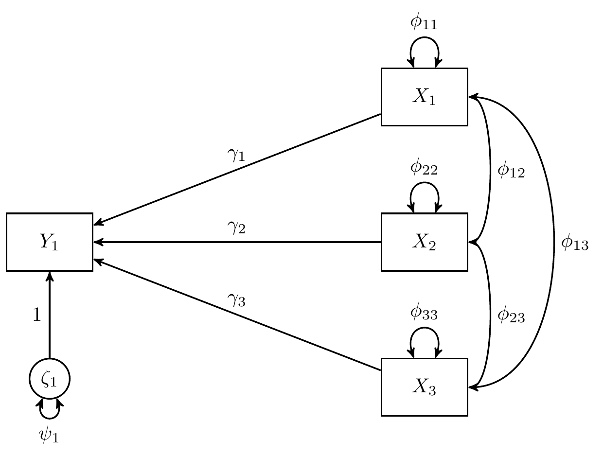
In this example, we use data from Kwan & Chan (2011) where child’s reading ability (\(Y_{1}\)) is regressed on parental occupational status (\(X_{1}\)), parental educational level (\(X_{2}\)), and child’s home possession (\(X_{3}\))

\[ Y_{1} = \alpha_{1} + \gamma_{1} X_{1} + \gamma_{2} X_{2} + \gamma_{3} X_{3} + \zeta_{1} . \]

Note that \(\zeta_{1}\) is the stochastic error term with expected value of zero and finite variance \(\psi_{1}\), \(\alpha_{1}\) is the intercept, and \(\gamma_{1}\), \(\gamma_{2}\), and \(\gamma_{3}\) are regression coefficients.

A Three-Regressor Multiple Regression Model (Covariance Structure)

covs
#>           Y1       X1      X2      X3
#> Y1 6088.8281 271.1429 49.5848 20.0337
#> X1  271.1429 226.2577 29.9232  4.8812
#> X2   49.5848  29.9232  9.0692  1.0312
#> X3   20.0337   4.8812  1.0312  0.8371
nobs
#> [1] 200

Model Specification

We regress Y1 on X1, X2, and X3.

model <- "
  Y1 ~ X1 + X2 + X3
"

Model Fitting

We can now fit the model using the sem() function from lavaan with mimic = "eqs" to ensure compatibility with results from Kwan & Chan (2011).

Note: We recommend setting fixed.x = FALSE when generating standardized estimates and confidence intervals to model the variances and covariances of the exogenous observed variables if they are assumed to be random. If fixed.x = TRUE, which is the default setting in lavaan, MC() will fix the variances and the covariances of the exogenous observed variables to the sample values.

fit <- sem(
  model = model, mimic = "eqs", fixed.x = FALSE,
  sample.cov = covs, sample.nobs = nobs
)

Standardized Monte Carlo Confidence Intervals

Standardized Monte Carlo Confidence intervals can be generated by passing the result of the MC() function to the MCStd() function.

unstd <- MC(fit, R = 20000L, alpha = 0.05)
MCStd(unstd, alpha = 0.05)
#> Standardized Monte Carlo Confidence Intervals
#>           est     se     R    2.5%  97.5%
#> Y1~X1  0.1207 0.0900 20000 -0.0589 0.2945
#> Y1~X2  0.0491 0.0913 20000 -0.1294 0.2286
#> Y1~X3  0.2194 0.0709 20000  0.0784 0.3562
#> Y1~~Y1 0.9002 0.0405 20000  0.8005 0.9579
#> X1~~X1 1.0000 0.0000 20000  1.0000 1.0000
#> X1~~X2 0.6606 0.0406 20000  0.5745 0.7348
#> X1~~X3 0.3547 0.0627 20000  0.2252 0.4715
#> X2~~X2 1.0000 0.0000 20000  1.0000 1.0000
#> X2~~X3 0.3743 0.0622 20000  0.2480 0.4901
#> X3~~X3 1.0000 0.0000 20000  1.0000 1.0000

References

Kwan, J. L. Y., & Chan, W. (2011). Comparing standardized coefficients in structural equation modeling: A model reparameterization approach. Behavior Research Methods, 43(3), 730–745. https://doi.org/10.3758/s13428-011-0088-6

Pesigan, I. J. A., & Cheung, S. F. (2023). Monte Carlo confidence intervals for the indirect effect with missing data. Behavior Research Methods. https://doi.org/10.3758/s13428-023-02114-4