Example 5: Composite Reliability
Ivan Jacob Agaloos Pesigan
2026-06-14
Source:vignettes/example-5-composite-reliability.Rmd
example-5-composite-reliability.RmdIn this example, the Monte Carlo method is used to generate confidence intervals for composite reliability using the Holzinger and Swineford (1939) data set.
data(HolzingerSwineford1939, package = "lavaan")The confirmatory factor analysis model for is given by
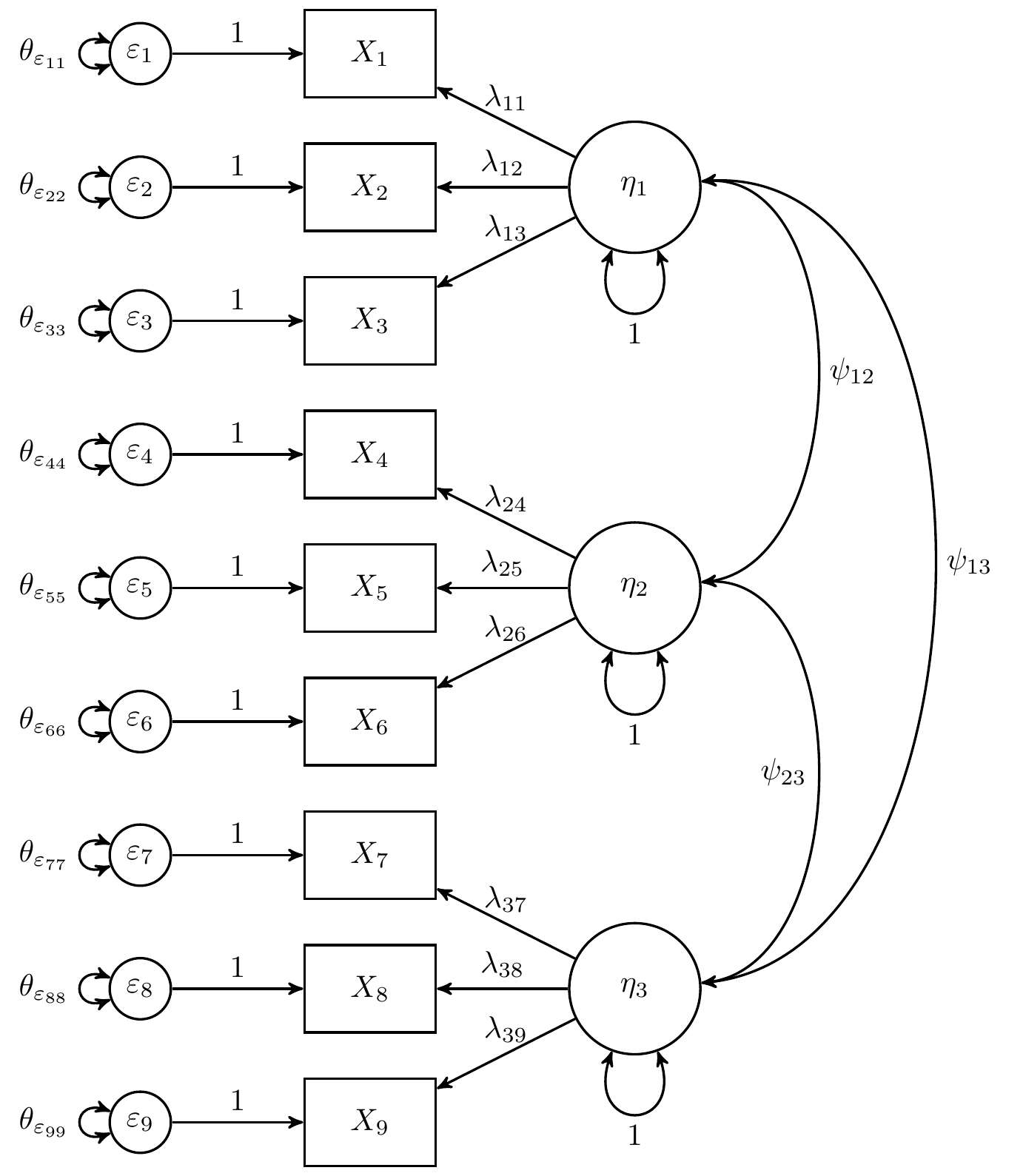
, , and are the latent factors. has three indicators , , and ; has three indicators , , and ; and has three indicators , , and . The variances of , , and are constrained to one.
Model Specification
Assuming that the latent variable variance is constrained to one, the omega total reliability coefficient is given by
where is the factor loading for item , is the residual variance for item , and is the number of items for a particular latent variable.
In the model specification below, the variances of the latent
variables eta1, eta2, and eta3
are constrained to one, all the relevant parameters are labeled
particularly the factor loadings and the error variances, and the omega
total reliability coefficient per latent variable are defined using the
:= operator.
model <- "
  # fix latent variable variances to 1
  eta1 ~~ 1 * eta1
  eta2 ~~ 1 * eta2
  eta3 ~~ 1 * eta3
  # factor loadings
  eta1 =~ NA * x1 + l11 * x1 + l12 * x2 + l13 * x3
  eta2 =~ NA * x4 + l24 * x4 + l25 * x5 + l26 * x6
  eta3 =~ NA * x7 + l37 * x7 + l38 * x8 + l39 * x9
  # error variances
  x1 ~~ t1 * x1
  x2 ~~ t2 * x2
  x3 ~~ t3 * x3
  x4 ~~ t4 * x4
  x5 ~~ t5 * x5
  x6 ~~ t6 * x6
  x7 ~~ t7 * x7
  x8 ~~ t8 * x8
  x9 ~~ t9 * x9
  # composite reliability
  omega1 := (l11 + l12 + l13)^2 / ((l11 + l12 + l13)^2 + (t1 + t2 + t3))
  omega2 := (l24 + l25 + l26)^2 / ((l24 + l25 + l26)^2 + (t4 + t5 + t6))
  omega3 := (l37 + l38 + l39)^2 / ((l37 + l38 + l39)^2 + (t7 + t8 + t9))
"
Model Fitting
We can now fit the model using the cfa() function from
lavaan.
fit <- cfa(model = model, data = HolzingerSwineford1939)Monte Carlo Confidence Intervals
The fit lavaan object can then be passed to
the MC() function to generate Monte Carlo confidence
intervals.
MC(fit, R = 20000L, alpha = 0.05)
#> Monte Carlo Confidence Intervals
#>               est     se     R   2.5%  97.5%
#> eta1~~eta1 1.0000 0.0000 20000 1.0000 1.0000
#> eta2~~eta2 1.0000 0.0000 20000 1.0000 1.0000
#> eta3~~eta3 1.0000 0.0000 20000 1.0000 1.0000
#> l11        0.8996 0.0806 20000 0.7391 1.0567
#> l12        0.4979 0.0770 20000 0.3474 0.6500
#> l13        0.6562 0.0745 20000 0.5089 0.8028
#> l24        0.9897 0.0566 20000 0.8785 1.1000
#> l25        1.1016 0.0627 20000 0.9801 1.2255
#> l26        0.9166 0.0533 20000 0.8110 1.0207
#> l37        0.6195 0.0693 20000 0.4844 0.7561
#> l38        0.7309 0.0654 20000 0.6026 0.8591
#> l39        0.6700 0.0655 20000 0.5426 0.7989
#> t1         0.5491 0.1140 20000 0.3264 0.7749
#> t2         1.1338 0.1032 20000 0.9323 1.3370
#> t3         0.8443 0.0916 20000 0.6643 1.0245
#> t4         0.3712 0.0477 20000 0.2783 0.4654
#> t5         0.4463 0.0592 20000 0.3310 0.5617
#> t6         0.3562 0.0430 20000 0.2726 0.4411
#> t7         0.7994 0.0816 20000 0.6413 0.9562
#> t8         0.4877 0.0737 20000 0.3427 0.6317
#> t9         0.5661 0.0708 20000 0.4253 0.7034
#> eta1~~eta2 0.4585 0.0640 20000 0.3347 0.5861
#> eta1~~eta3 0.4705 0.0727 20000 0.3282 0.6132
#> eta2~~eta3 0.2830 0.0688 20000 0.1480 0.4182
#> omega1     0.6253 0.0363 20000 0.5488 0.6910
#> omega2     0.8852 0.0116 20000 0.8599 0.9058
#> omega3     0.6878 0.0312 20000 0.6215 0.7436