Example 3: The Latent Variable Simple Mediation Model
Ivan Jacob Agaloos Pesigan
2026-06-14
Source:vignettes/example-3-latent.Rmd
example-3-latent.RmdIn this example, the Monte Carlo method is used to generate
confidence intervals for the indirect effects in a simple mediation
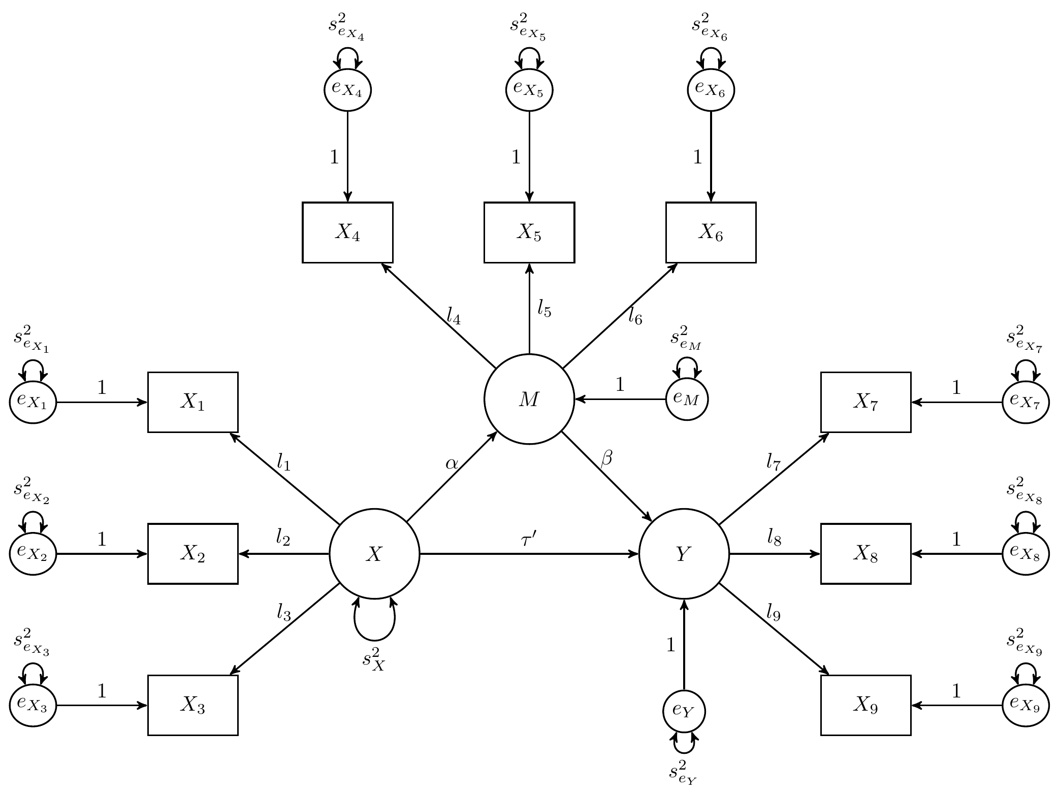
model with latent variables. X, M, and
Y are latent variables with three indicators each where
X is the predictor, M is the mediator, and
Y is the dependent variable.
Model Specification
The indirect effect is defined by the product of the slopes of paths
X to M labeled as a and
M to Y labeled as b. In this
example, we are interested in the confidence intervals of
indirect defined as the product of a and
b using the := operator in the
lavaan model syntax.
model <- "
  X =~ x1 + x2 + x3
  M =~ x4 + x5 + x6
  Y =~ x7 + x8 + x9
  M ~ a * X
  Y ~ b * M
  indirect := a * b
"
Model Fitting
We can now fit the model using the sem() function from
lavaan using the Holzinger and Swineford (1939) data
set.
df <- lavaan::HolzingerSwineford1939
fit <- sem(data = df, model = model)
Monte Carlo Confidence Intervals
The fit lavaan object can then be passed to
the MC() function from semmcci to generate
Monte Carlo confidence intervals.
MC(fit, R = 20000L, alpha = 0.05)
#> Monte Carlo Confidence Intervals
#>             est     se     R   2.5%  97.5%
#> X=~x1    1.0000 0.0000 20000 1.0000 1.0000
#> X=~x2    0.5554 0.1044 20000 0.3539 0.7599
#> X=~x3    0.7045 0.1176 20000 0.4739 0.9374
#> M=~x4    1.0000 0.0000 20000 1.0000 1.0000
#> M=~x5    1.1106 0.0648 20000 0.9837 1.2391
#> M=~x6    0.9268 0.0555 20000 0.8181 1.0368
#> Y=~x7    1.0000 0.0000 20000 1.0000 1.0000
#> Y=~x8    1.1482 0.1647 20000 0.8245 1.4665
#> Y=~x9    0.8854 0.1241 20000 0.6417 1.1283
#> a        0.5107 0.0954 20000 0.3265 0.6999
#> b        0.1884 0.0517 20000 0.0873 0.2888
#> x1~~x1   0.5320 0.1296 20000 0.2791 0.7848
#> x2~~x2   1.1269 0.1033 20000 0.9253 1.3276
#> x3~~x3   0.8647 0.0952 20000 0.6794 1.0512
#> x4~~x4   0.3714 0.0476 20000 0.2783 0.4653
#> x5~~x5   0.4519 0.0582 20000 0.3385 0.5655
#> x6~~x6   0.3551 0.0429 20000 0.2705 0.4384
#> x7~~x7   0.7309 0.0833 20000 0.5679 0.8953
#> x8~~x8   0.4257 0.0828 20000 0.2656 0.5888
#> x9~~x9   0.6605 0.0710 20000 0.5207 0.8008
#> X~~X     0.8264 0.1589 20000 0.5123 1.1396
#> M~~M     0.7638 0.0973 20000 0.5716 0.9556
#> Y~~Y     0.4175 0.0893 20000 0.2418 0.5900
#> indirect 0.0962 0.0319 20000 0.0399 0.1641
Standardized Monte Carlo Confidence Intervals
Standardized Monte Carlo Confidence intervals can be generated by
passing the result of the MC() function to the
MCStd() function.
MCStd(unstd, alpha = 0.05)
#> Standardized Monte Carlo Confidence Intervals
#>             est     se     R   2.5%  97.5%
#> X=~x1    0.7800 0.0629 20000 0.6418 0.8916
#> X=~x2    0.4295 0.0614 20000 0.2969 0.5391
#> X=~x3    0.5672 0.0602 20000 0.4325 0.6688
#> M=~x4    0.8515 0.0231 20000 0.8023 0.8925
#> M=~x5    0.8531 0.0227 20000 0.8045 0.8938
#> M=~x6    0.8385 0.0235 20000 0.7885 0.8799
#> Y=~x7    0.6183 0.0543 20000 0.4991 0.7132
#> Y=~x8    0.7639 0.0553 20000 0.6409 0.8575
#> Y=~x9    0.5910 0.0545 20000 0.4750 0.6876
#> a        0.4691 0.0646 20000 0.3302 0.5844
#> b        0.2772 0.0697 20000 0.1351 0.4109
#> x1~~x1   0.3917 0.0964 20000 0.2050 0.5880
#> x2~~x2   0.8155 0.0515 20000 0.7094 0.9119
#> x3~~x3   0.6783 0.0664 20000 0.5527 0.8129
#> x4~~x4   0.2750 0.0391 20000 0.2035 0.3563
#> x5~~x5   0.2722 0.0386 20000 0.2011 0.3527
#> x6~~x6   0.2969 0.0391 20000 0.2258 0.3782
#> x7~~x7   0.6177 0.0658 20000 0.4913 0.7509
#> x8~~x8   0.4165 0.0829 20000 0.2647 0.5892
#> x9~~x9   0.6507 0.0635 20000 0.5272 0.7744
#> X~~X     1.0000 0.0000 20000 1.0000 1.0000
#> M~~M     0.7799 0.0593 20000 0.6585 0.8910
#> Y~~Y     0.9231 0.0388 20000 0.8312 0.9818
#> indirect 0.1301 0.0377 20000 0.0580 0.2058