Example 2: The Serial Mediation Model
Ivan Jacob Agaloos Pesigan
2026-06-14
Source:vignettes/example-2-serial.Rmd
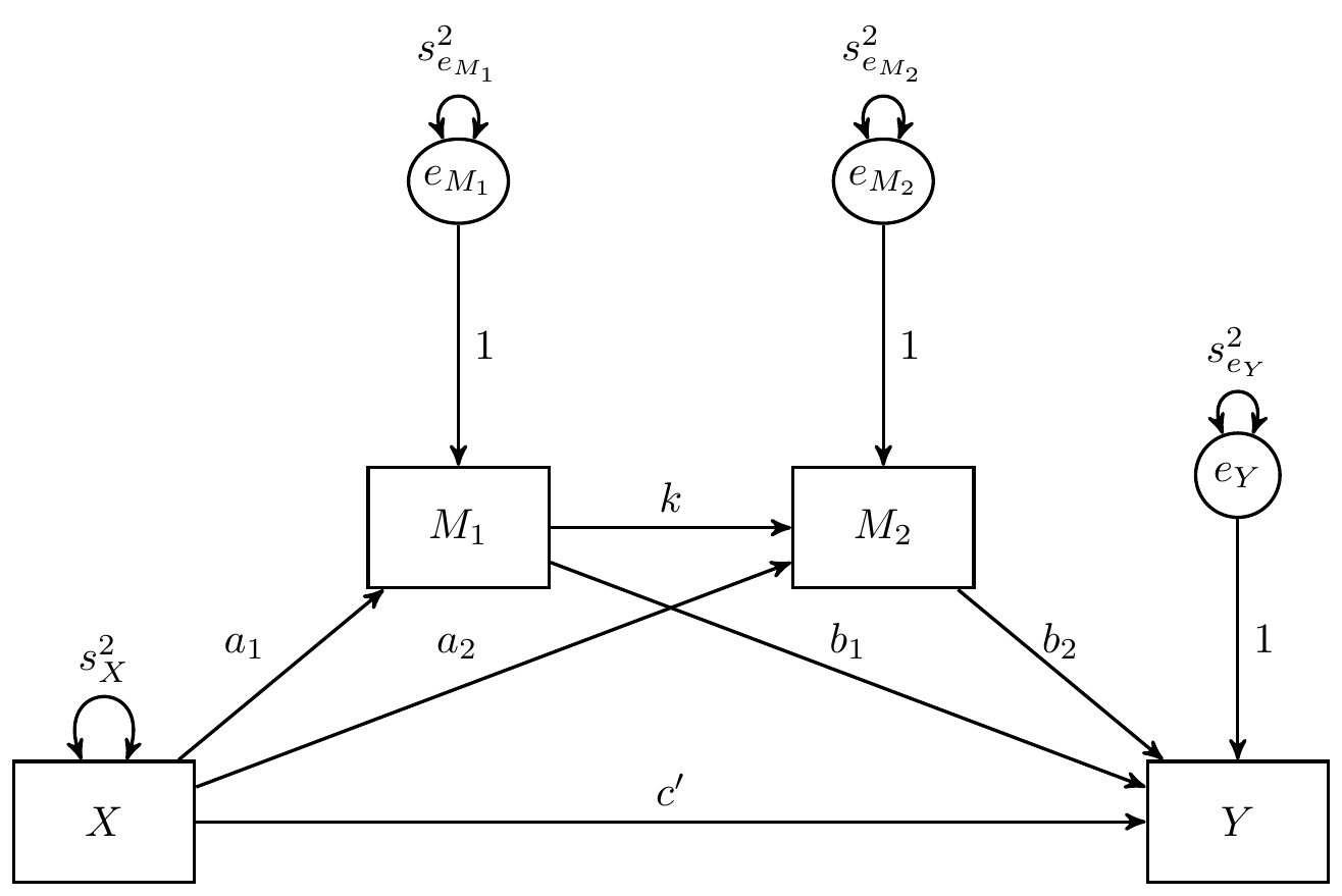
example-2-serial.RmdIn this example, the Monte Carlo method is used to generate
confidence intervals for the indirect effects in a serial mediation
model with two mediators where X is the predictor,
M1 is the first mediator, M2 is the second
mediator, and Y is the dependent variable.
Data
summary(df)
#>        X                  M1                 M2                 Y
#>  Min.   :-3.37174   Min.   :-3.22690   Min.   :-4.33590   Min.   :-4.29020
#>  1st Qu.:-0.67546   1st Qu.:-0.73709   1st Qu.:-0.82188   1st Qu.:-0.86035
#>  Median :-0.01313   Median :-0.01651   Median :-0.03903   Median :-0.02704
#>  Mean   :-0.02582   Mean   :-0.01823   Mean   :-0.01620   Mean   :-0.03338
#>  3rd Qu.: 0.66401   3rd Qu.: 0.72825   3rd Qu.: 0.80016   3rd Qu.: 0.81721
#>  Max.   : 3.49530   Max.   : 3.69001   Max.   : 3.65147   Max.   : 4.05239
colMeans(df)
#>           X          M1          M2           Y
#> -0.02582443 -0.01823021 -0.01619576 -0.03337865
var(df)
#>            X        M1        M2         Y
#> X  1.0050488 0.5123920 0.3848638 0.3333458
#> M1 0.5123920 1.2334461 0.6645408 0.5108946
#> M2 0.3848638 0.6645408 1.4321822 0.8012638
#> Y  0.3333458 0.5108946 0.8012638 1.4504417
Model Specification
We can define several indirect effects in this example:
These indirect effects are defined using the := operator
in the lavaan model syntax.
model <- "
  Y ~ cp * X + b1 * M1 + b2 * M2
  M2 ~ a2 * X + k * M1
  M1 ~ a1 * X
  # X -> M1 -> M2 -> Y
  a1kb2 := a1 * k * b2
  # X -> M1 -> M2
  a1k := a1 * k
  # X -> M1 -> Y
  a2b2 := a2 * b2
  # M1 -> M2 -> Y
  kb2 := k * b2
"
Model Fitting
fit <- sem(data = df, model = model)Monte Carlo Confidence Intervals
The fit lavaan object can then be passed to
the MC() function from semmcci to generate
Monte Carlo confidence intervals.
MC(fit, R = 20000L, alpha = 0.05)
#> Monte Carlo Confidence Intervals
#>           est     se     R   2.5%  97.5%
#> cp     0.0868 0.0354 20000 0.0172 0.1567
#> b1     0.1190 0.0352 20000 0.0501 0.1874
#> b2     0.4809 0.0304 20000 0.4219 0.5406
#> a2     0.1373 0.0367 20000 0.0657 0.2098
#> k      0.4817 0.0328 20000 0.4175 0.5463
#> a1     0.5098 0.0310 20000 0.4496 0.5713
#> Y~~Y   0.9744 0.0439 20000 0.8885 1.0603
#> M2~~M2 1.0581 0.0477 20000 0.9641 1.1510
#> M1~~M1 0.9712 0.0431 20000 0.8872 1.0563
#> X~~X   1.0040 0.0000 20000 1.0040 1.0040
#> a1kb2  0.1181 0.0132 20000 0.0936 0.1456
#> a1k    0.2456 0.0225 20000 0.2029 0.2913
#> a2b2   0.0660 0.0182 20000 0.0312 0.1026
#> kb2    0.2317 0.0216 20000 0.1911 0.2754
Standardized Monte Carlo Confidence Intervals
Standardized Monte Carlo Confidence intervals can be generated by
passing the result of the MC() function to the
MCStd() function.
Note: We recommend setting
fixed.x = FALSEwhen generating standardized estimates and confidence intervals to model the variances and covariances of the exogenous observed variables if they are assumed to be random. Iffixed.x = TRUE, which is the default setting inlavaan,MC()will fix the variances and the covariances of the exogenous observed variables to the sample values.
MCStd(unstd, alpha = 0.05)
#> Standardized Monte Carlo Confidence Intervals
#>           est     se     R   2.5%  97.5%
#> cp     0.0723 0.0290 20000 0.0158 0.1300
#> b1     0.1098 0.0317 20000 0.0474 0.1715
#> b2     0.4779 0.0274 20000 0.4236 0.5310
#> a2     0.1151 0.0306 20000 0.0544 0.1745
#> k      0.4470 0.0282 20000 0.3908 0.5018
#> a1     0.4602 0.0249 20000 0.4108 0.5084
#> Y~~Y   0.6725 0.0243 20000 0.6224 0.7185
#> M2~~M2 0.7396 0.0238 20000 0.6907 0.7843
#> M1~~M1 0.7882 0.0229 20000 0.7415 0.8312
#> X~~X   1.0000 0.0000 20000 1.0000 1.0000
#> a1kb2  0.0983 0.0104 20000 0.0790 0.1195
#> a1k    0.2057 0.0176 20000 0.1718 0.2406
#> a2b2   0.0550 0.0149 20000 0.0257 0.0845
#> kb2    0.2136 0.0188 20000 0.1778 0.2510