Example 1: The Simple Mediation Model

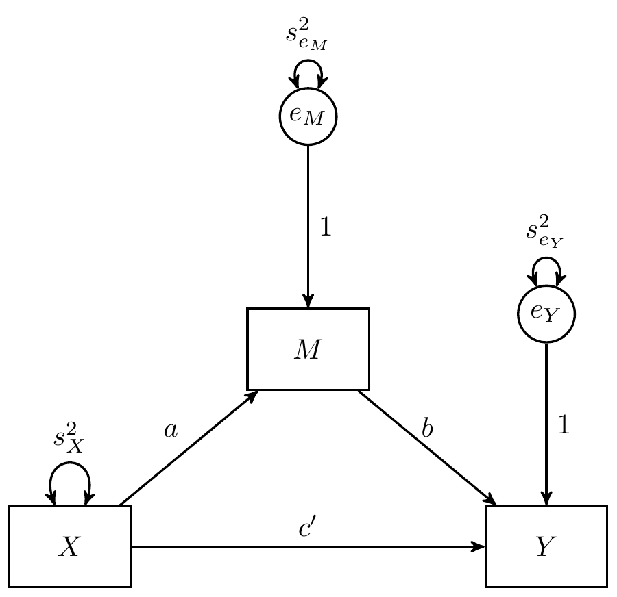
In this example, the Monte Carlo method is used to generate confidence intervals for the indirect effect in a simple mediation model where variable X has an effect on variable Y, through a mediating variable M. This mediating or indirect effect is a product of path coefficients from the fitted model.

$The Simple Mediation Model$

The Simple Mediation Model

library(semmcci)
library(lavaan)

Data

summary(df)
#>        X                   M                   Y           
#>  Min.   :-3.199558   Min.   :-3.371276   Min.   :-3.61432  
#>  1st Qu.:-0.636035   1st Qu.:-0.692640   1st Qu.:-0.66146  
#>  Median : 0.011377   Median : 0.007125   Median :-0.04726  
#>  Mean   :-0.003207   Mean   :-0.023968   Mean   :-0.01677  
#>  3rd Qu.: 0.651951   3rd Qu.: 0.647363   3rd Qu.: 0.62640  
#>  Max.   : 3.470910   Max.   : 2.963216   Max.   : 3.09950
colMeans(df)
#>            X            M            Y 
#> -0.003206987 -0.023968103 -0.016774294
var(df)
#>           X         M         Y
#> X 1.0600162 0.5108780 0.5069458
#> M 0.5108780 0.9996606 0.6272104
#> Y 0.5069458 0.6272104 0.9837255

Model Specification

The indirect effect is defined by the product of the slopes of paths X to M labeled as a and M to Y labeled as b. In this example, we are interested in the confidence intervals of indirect defined as the product of a and b using the := operator in the lavaan model syntax.

model <- "
  Y ~ cp * X + b * M
  M ~ a * X
  indirect := a * b
  direct := cp
  total := cp + (a * b)
"

Model Fitting

We can now fit the model using the sem() function from lavaan.

fit <- sem(data = df, model = model)

Monte Carlo Confidence Intervals

The fit lavaan object can then be passed to the MC() function to generate Monte Carlo confidence intervals.

MC(fit, R = 20000L, alpha = 0.05)
#> Monte Carlo Confidence Intervals
#>             est     se     R   2.5%  97.5%
#> cp       0.2333 0.0264 20000 0.1819 0.2849
#> b        0.5082 0.0272 20000 0.4553 0.5613
#> a        0.4820 0.0264 20000 0.4302 0.5340
#> Y~~Y     0.5462 0.0244 20000 0.4979 0.5944
#> M~~M     0.7527 0.0339 20000 0.6858 0.8187
#> X~~X     1.0590 0.0000 20000 1.0590 1.0590
#> indirect 0.2449 0.0187 20000 0.2094 0.2831
#> direct   0.2333 0.0264 20000 0.1819 0.2849
#> total    0.4782 0.0265 20000 0.4261 0.5306

Standardized Monte Carlo Confidence Intervals

Standardized Monte Carlo Confidence intervals can be generated by passing the result of the MC() function to the MCStd() function.

Note: We recommend setting fixed.x = FALSE when generating standardized estimates and confidence intervals to model the variances and covariances of the exogenous observed variables if they are assumed to be random. If fixed.x = TRUE, which is the default setting in lavaan, MC() will fix the variances and the covariances of the exogenous observed variables to the sample values.

fit <- sem(data = df, model = model, fixed.x = FALSE)
unstd <- MC(fit, R = 20000L, alpha = 0.05)

MCStd(unstd, alpha = 0.05)
#> Standardized Monte Carlo Confidence Intervals
#>             est     se     R   2.5%  97.5%
#> cp       0.2422 0.0266 20000 0.1897 0.2941
#> b        0.5123 0.0247 20000 0.4636 0.5605
#> a        0.4963 0.0240 20000 0.4476 0.5416
#> Y~~Y     0.5558 0.0236 20000 0.5089 0.6015
#> M~~M     0.7537 0.0238 20000 0.7066 0.7996
#> X~~X     1.0000 0.0000 20000 1.0000 1.0000
#> indirect 0.2542 0.0177 20000 0.2199 0.2891
#> direct   0.2422 0.0266 20000 0.1897 0.2941
#> total    0.4964 0.0239 20000 0.4477 0.5417

Standardized Monte Carlo Confidence Intervals - An Alternative Approach

In this example, confidence intervals for the standardized indirect effect are generated by specifying the standardized indirect effect as a derived parameter using the := operator. The standardized indirect effect in a simple mediation model involves paths $a$ and $b$, and the standard deviations of $X$ and $Y$. It is given by

\[ a b \frac{s_X}{s_Y} \]

where

\[ s_X = \sqrt{ s_{X}^{2} } \]

and

\[ s_Y = \sqrt{ c^{\prime 2} s_{X}^{2} + a^2 b^2 s_{X}^{2} + b^2 s_{e_{M}}^{2} + 2 c^{\prime} b a s_{X}^{2} + s_{e_{Y}}^{2} } \]

where

$s_{e_{Y}}^{2}$ and $s_{e_{M}}^{2}$ are the residual variances in the regression equations.

The standardized indirect effect can be defined using the := operator and the named parameters in the model.

model <- "
  Y ~ cp * X + b * M
  M ~ a * X
  X ~~ s2_X * X
  M ~~ s2_em * M
  Y ~~ s2_ey * Y
  indirect_std := a * b * (
    sqrt(s2_X) / sqrt(
      (
        cp^2 * s2_X + a^2 * b^2 * s2_X
      ) + (
        b^2 * s2_em
      ) + (
        2 * cp * b * a * s2_X
      ) + s2_ey
    )
  )
"

fit <- sem(data = df, model = model, fixed.x = FALSE)

The row indirect_std corresponds to the confidence intervals for the standardized indirect effect.

MC(fit, R = 20000L, alpha = 0.05)
#> Monte Carlo Confidence Intervals
#>                 est     se     R   2.5%  97.5%
#> cp           0.2333 0.0263 20000 0.1810 0.2838
#> b            0.5082 0.0270 20000 0.4553 0.5613
#> a            0.4820 0.0264 20000 0.4309 0.5338
#> s2_X         1.0590 0.0472 20000 0.9648 1.1504
#> s2_em        0.7527 0.0339 20000 0.6865 0.8192
#> s2_ey        0.5462 0.0243 20000 0.4987 0.5940
#> indirect_std 0.2542 0.0174 20000 0.2206 0.2888

References

Pesigan, I. J. A., & Cheung, S. F. (2023). Monte Carlo confidence intervals for the indirect effect with missing data. Behavior Research Methods. https://doi.org/10.3758/s13428-023-02114-4

Ivan Jacob Agaloos Pesigan