Benchmark: Comparing the Monte Carlo Method with Nonparametric Bootstrapping (MI)
Ivan Jacob Agaloos Pesigan
2026-06-13
Source:vignettes/benchmark-mi.Rmd
benchmark-mi.RmdWe compare the Monte Carlo (MC) method with nonparametric bootstrapping (NB) using the simple mediation model with missing data using multiple imputation. One advantage of MC over NB is speed. This is because the model is only fitted once in MC whereas it is fitted many times in NB.
Data
n <- 1000
a <- 0.50
b <- 0.50
cp <- 0.25
s2_em <- 1 - a^2
s2_ey <- 1 - cp^2 - a^2 * b^2 - b^2 * s2_em - 2 * cp * a * b
em <- rnorm(n = n, mean = 0, sd = sqrt(s2_em))
ey <- rnorm(n = n, mean = 0, sd = sqrt(s2_ey))
X <- rnorm(n = n)
M <- a * X + em
Y <- cp * X + b * M + ey
df <- data.frame(X, M, Y)

# Create data set with missing values.

miss <- sample(1:dim(df)[1], 300)
df[miss[1:100], "X"] <- NA
df[miss[101:200], "M"] <- NA
df[miss[201:300], "Y"] <- NA
Multiple Imputation
Perform the appropriate multiple imputation approach to deal with missing values. In this example, we impute multivariate missing data under the normal model.
mi <- amelia(
  x = df,
  m = 5L,
  p2s = 0
)
Model Specification
The indirect effect is defined by the product of the slopes of paths
X to M labeled as a and
M to Y labeled as b. In this
example, we are interested in the confidence intervals of
indirect defined as the product of a and
b using the := operator in the
lavaan model syntax.
model <- "
  Y ~ cp * X + b * M
  M ~ a * X
  X ~~ X
  indirect := a * b
  direct := cp
  total := cp + (a * b)
"
Model Fitting
We can now fit the model using the sem() function from
lavaan. We do not need to deal with missing values in this
stage.
fit <- sem(data = df, model = model)Monte Carlo Confidence Intervals (Multiple Imputation)
The fit lavaan object and mi
mids object can then be passed to the MCMI()
function from semmcci to generate Monte Carlo confidence
intervals using multiple imputation as described in Pesigan and Cheung
(2024).
MCMI(fit, R = 100L, alpha = 0.05, mi = mi)
#> Monte Carlo Confidence Intervals (Multiple Imputation Estimates)
#>             est     se   R   2.5%  97.5%
#> cp       0.2274 0.0295 100 0.1787 0.2818
#> b        0.5192 0.0342 100 0.4534 0.5839
#> a        0.4790 0.0281 100 0.4249 0.5266
#> X~~X     1.0613 0.0443 100 0.9775 1.1328
#> Y~~Y     0.5439 0.0244 100 0.5010 0.5911
#> M~~M     0.7642 0.0397 100 0.7048 0.8397
#> indirect 0.2486 0.0189 100 0.2103 0.2755
#> direct   0.2274 0.0295 100 0.1787 0.2818
#> total    0.4760 0.0288 100 0.4243 0.5329
Nonparametric Bootstrap Confidence Intervals (Multiple Imputation)
Nonparametric bootstrap confidence intervals can be generated in
bmemLavaan using the following.
summary(
  bmemLavaan::bmem(data = df, model = model, method = "mi", boot = 100L, m = 5L)
)
#>
#> Estimate method:                          multiple imputation
#> Sample size:                              1000
#> Number of request bootstrap draws:        100
#> Number of successful bootstrap draws:     100
#> Type of confidence interval:              perc
#>
#> Values of statistics:
#>
#>                      Value      SE      2.5%     97.5%
#>   chisq               0.000    0.000    0.000    0.000
#>   GFI                 1.000    0.000    1.000    1.000
#>   AGFI                1.000    0.000    1.000    1.000
#>   RMSEA               0.000    0.000    0.000    0.000
#>   NFI                 1.000    0.000    1.000    1.000
#>   NNFI                1.000    0.000    1.000    1.000
#>   CFI                 1.000    0.000    1.000    1.000
#>   BIC                 7742.967 81.777   7575.258 7857.675
#>   SRMR                0.000    0.000    0.000    0.000
#>
#> Estimation of parameters:
#>
#>                      Estimate   SE      2.5%     97.5%
#> Regressions:
#>   Y ~
#>     X        (cp)     0.234    0.030    0.176    0.296
#>     M         (b)     0.513    0.032    0.460    0.570
#>   M ~
#>     X         (a)     0.476    0.030    0.426    0.540
#>
#> Variances:
#>     X                 1.057    0.046    0.950    1.144
#>     Y                 0.556    0.027    0.488    0.600
#>     M                 0.755    0.035    0.684    0.813
#>
#>
#>
#> Defined parameters:
#>     a*b    (indr)     0.244    0.020    0.206    0.285
#>     cp     (drct)     0.234    0.030    0.176    0.296
#>     cp+(*) (totl)     0.479    0.030    0.428    0.539
Benchmark
benchmark_mi_01 <- microbenchmark(
MC = {
fit <- sem(
data = df,
model = model
)
mi <- Amelia::amelia(
x = df,
m = m,
p2s = 0
)
MCMI(
fit,
R = R,
decomposition = "chol",
pd = FALSE,
mi = mi
)
},
NB = bmemLavaan::bmem(
data = df,
model = model,
method = "mi",
boot = B,
m = m
),
times = 10
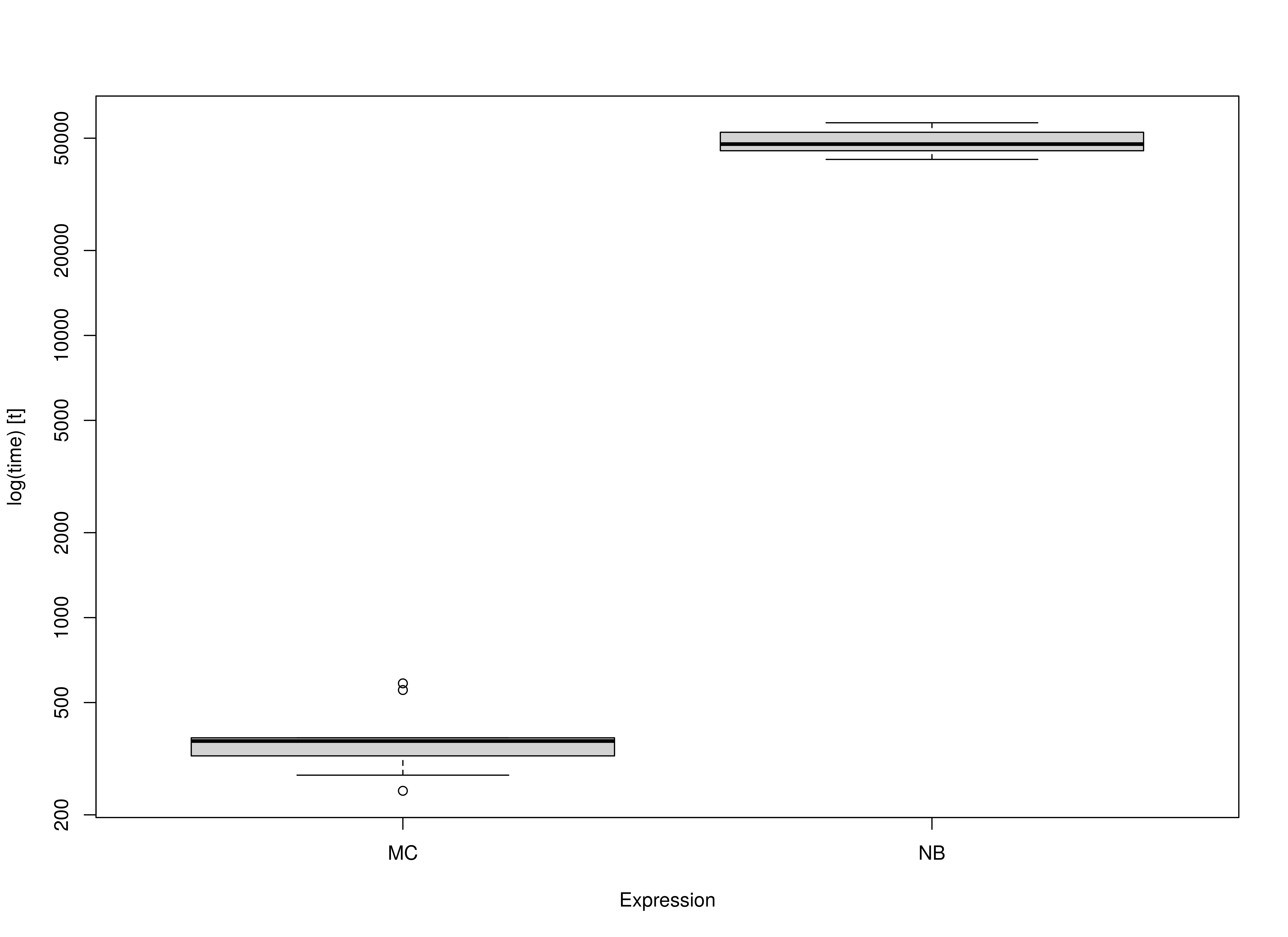
)Summary of Benchmark Results
summary(benchmark_mi_01, unit = "ms")
#>   expr        min        lq       mean     median         uq        max neval
#> 1   MC   250.0695   256.085   262.3459   261.9223   268.0928   274.7592    10
#> 2   NB 25835.1467 26228.463 26413.2280 26438.3644 26620.1658 26879.2109    10
Summary of Benchmark Results Relative to the Faster Method
summary(benchmark_mi_01, unit = "relative")
#>   expr      min       lq     mean   median       uq      max neval
#> 1   MC   1.0000   1.0000   1.0000   1.0000  1.00000  1.00000    10
#> 2   NB 103.3119 102.4209 100.6809 100.9397 99.29458 97.82824    10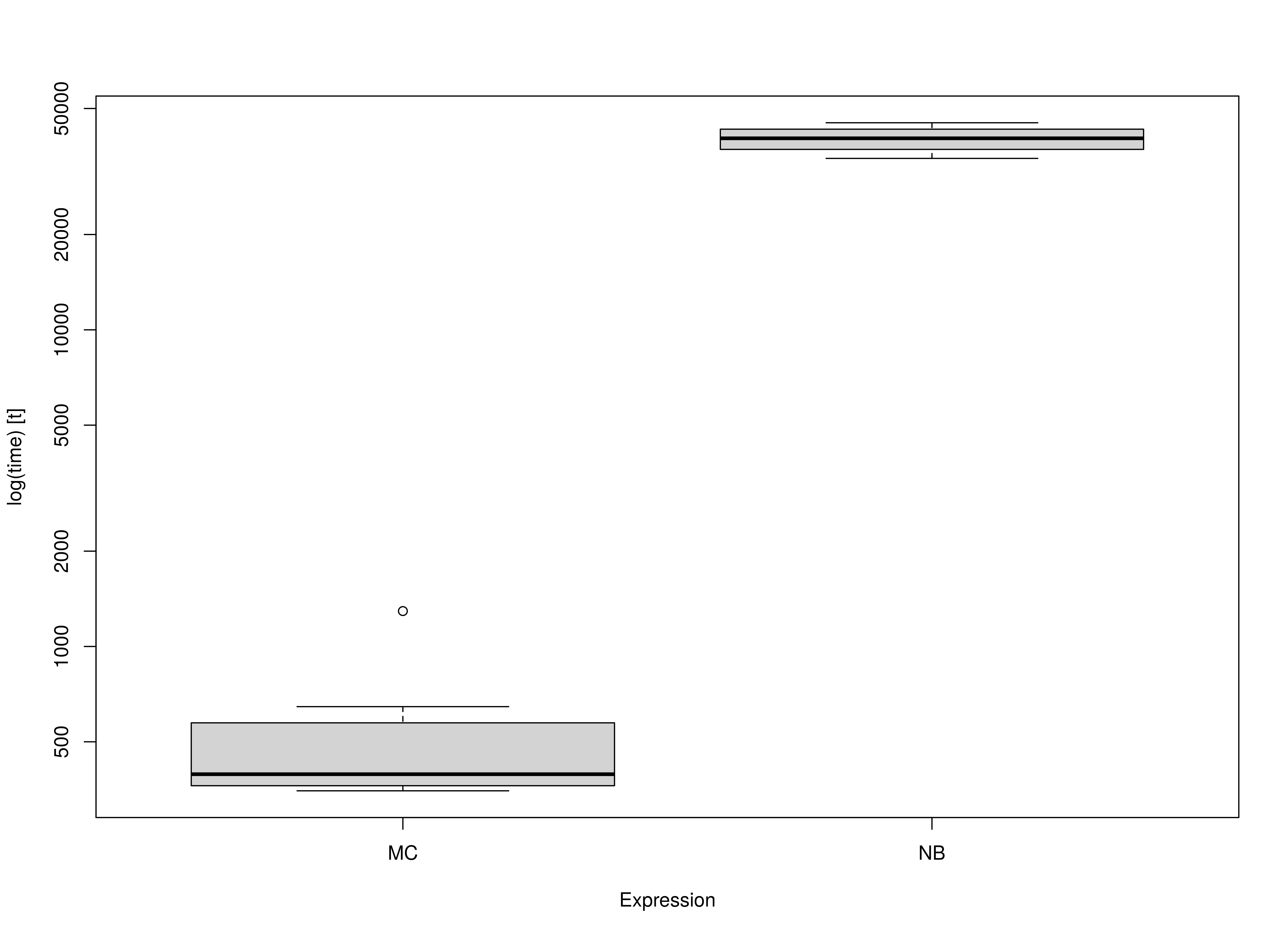
Benchmark - Monte Carlo Method with Precalculated Estimates and Multiple Imputation
fit <- sem(
  data = df,
  model = model
)
mi <- Amelia::amelia(
  x = df,
  m = m,
  p2s = 0
)
benchmark_mi_02 <- microbenchmark(
  MC = MCMI(
    fit,
    R = R,
    decomposition = "chol",
    pd = FALSE,
    mi = mi
  ),
  NB = bmemLavaan::bmem(
    data = df,
    model = model,
    method = "mi",
    boot = B,
    m = m
  ),
  times = 10
)
Summary of Benchmark Results
summary(benchmark_mi_02, unit = "ms")
#>   expr        min         lq       mean     median         uq        max neval
#> 1   MC   183.9795   189.3579   213.6721   197.1329   201.1853   385.8201    10
#> 2   NB 25685.9663 26099.4942 26295.6417 26302.2223 26648.0516 26955.0059    10
Summary of Benchmark Results Relative to the Faster Method
summary(benchmark_mi_02, unit = "relative")
#>   expr      min       lq     mean   median       uq      max neval
#> 1   MC   1.0000   1.0000   1.0000   1.0000   1.0000  1.00000    10
#> 2   NB 139.6132 137.8315 123.0654 133.4238 132.4552 69.86418    10