Benchmark: Comparing the Monte Carlo Method with Nonparametric Bootstrapping (FIML)
Ivan Jacob Agaloos Pesigan
2026-06-13
Source:vignettes/benchmark-fiml.Rmd
benchmark-fiml.RmdWe compare the Monte Carlo (MC) method with nonparametric bootstrapping (NB) using the simple mediation model with missing data using full-information maximum likelihood. One advantage of MC over NB is speed. This is because the model is only fitted once in MC whereas it is fitted many times in NB.
Data
n <- 1000
a <- 0.50
b <- 0.50
cp <- 0.25
s2_em <- 1 - a^2
s2_ey <- 1 - cp^2 - a^2 * b^2 - b^2 * s2_em - 2 * cp * a * b
em <- rnorm(n = n, mean = 0, sd = sqrt(s2_em))
ey <- rnorm(n = n, mean = 0, sd = sqrt(s2_ey))
X <- rnorm(n = n)
M <- a * X + em
Y <- cp * X + b * M + ey
df <- data.frame(X, M, Y)

# Create data set with missing values.

miss <- sample(1:dim(df)[1], 300)
df[miss[1:100], "X"] <- NA
df[miss[101:200], "M"] <- NA
df[miss[201:300], "Y"] <- NA
Model Specification
The indirect effect is defined by the product of the slopes of paths
X to M labeled as a and
M to Y labeled as b. In this
example, we are interested in the confidence intervals of
indirect defined as the product of a and
b using the := operator in the
lavaan model syntax.
model <- "
  Y ~ cp * X + b * M
  M ~ a * X
  X ~~ X
  indirect := a * b
  direct := cp
  total := cp + (a * b)
"
Model Fitting
We can now fit the model using the sem() function from
lavaan. We are using missing = "fiml" to
handle missing data in lavaan.
fit <- sem(data = df, model = model)Monte Carlo Confidence Intervals
The fit lavaan object can then be passed to
the MC() function from semmcci to generate
Monte Carlo confidence intervals.
MC(fit, R = 100L, alpha = 0.05)
#> Monte Carlo Confidence Intervals
#>             est     se   R   2.5%  97.5%
#> cp       0.2419 0.0332 100 0.1792 0.3070
#> b        0.5166 0.0308 100 0.4580 0.5785
#> a        0.4989 0.0319 100 0.4448 0.5615
#> X~~X     1.0951 0.0621 100 0.9856 1.2026
#> Y~~Y     0.5796 0.0307 100 0.5257 0.6413
#> M~~M     0.8045 0.0464 100 0.7325 0.9106
#> indirect 0.2577 0.0210 100 0.2234 0.3031
#> direct   0.2419 0.0332 100 0.1792 0.3070
#> total    0.4996 0.0322 100 0.4550 0.5681
Nonparametric Bootstrap Confidence Intervals
Nonparametric bootstrap confidence intervals can be generated in
lavaan using the following.
parameterEstimates(
  sem(
    data = df,
    model = model,
    missing = "fiml",
    se = "bootstrap",
    bootstrap = 100L
  )
)
#>         lhs op      rhs    label    est    se      z pvalue ci.lower ci.upper
#> 1         Y  ~        X       cp  0.234 0.030  7.721  0.000    0.169    0.287
#> 2         Y  ~        M        b  0.511 0.035 14.704  0.000    0.442    0.585
#> 3         M  ~        X        a  0.481 0.028 17.117  0.000    0.425    0.532
#> 4         X ~~        X           1.059 0.049 21.539  0.000    0.979    1.148
#> 5         Y ~~        Y           0.554 0.029 19.264  0.000    0.490    0.607
#> 6         M ~~        M           0.756 0.032 23.389  0.000    0.693    0.820
#> 7         Y ~1                   -0.013 0.027 -0.473  0.636   -0.065    0.056
#> 8         M ~1                   -0.022 0.030 -0.744  0.457   -0.077    0.044
#> 9         X ~1                    0.002 0.036  0.069  0.945   -0.072    0.074
#> 10 indirect :=      a*b indirect  0.246 0.021 11.534  0.000    0.202    0.286
#> 11   direct :=       cp   direct  0.234 0.030  7.721  0.000    0.169    0.287
#> 12    total := cp+(a*b)    total  0.479 0.030 16.081  0.000    0.417    0.547
Benchmark
Arguments
| Variables | Values | Notes |
|---|---|---|
| R | 1000 | Number of Monte Carlo replications. |
| B | 1000 | Number of bootstrap samples. |
benchmark_fiml_01 <- microbenchmark(
MC = {
fit <- sem(
data = df,
model = model,
missing = "fiml"
)
MC(
fit,
R = R,
decomposition = "chol",
pd = FALSE
)
},
NB = sem(
data = df,
model = model,
missing = "fiml",
se = "bootstrap",
bootstrap = B
),
times = 10
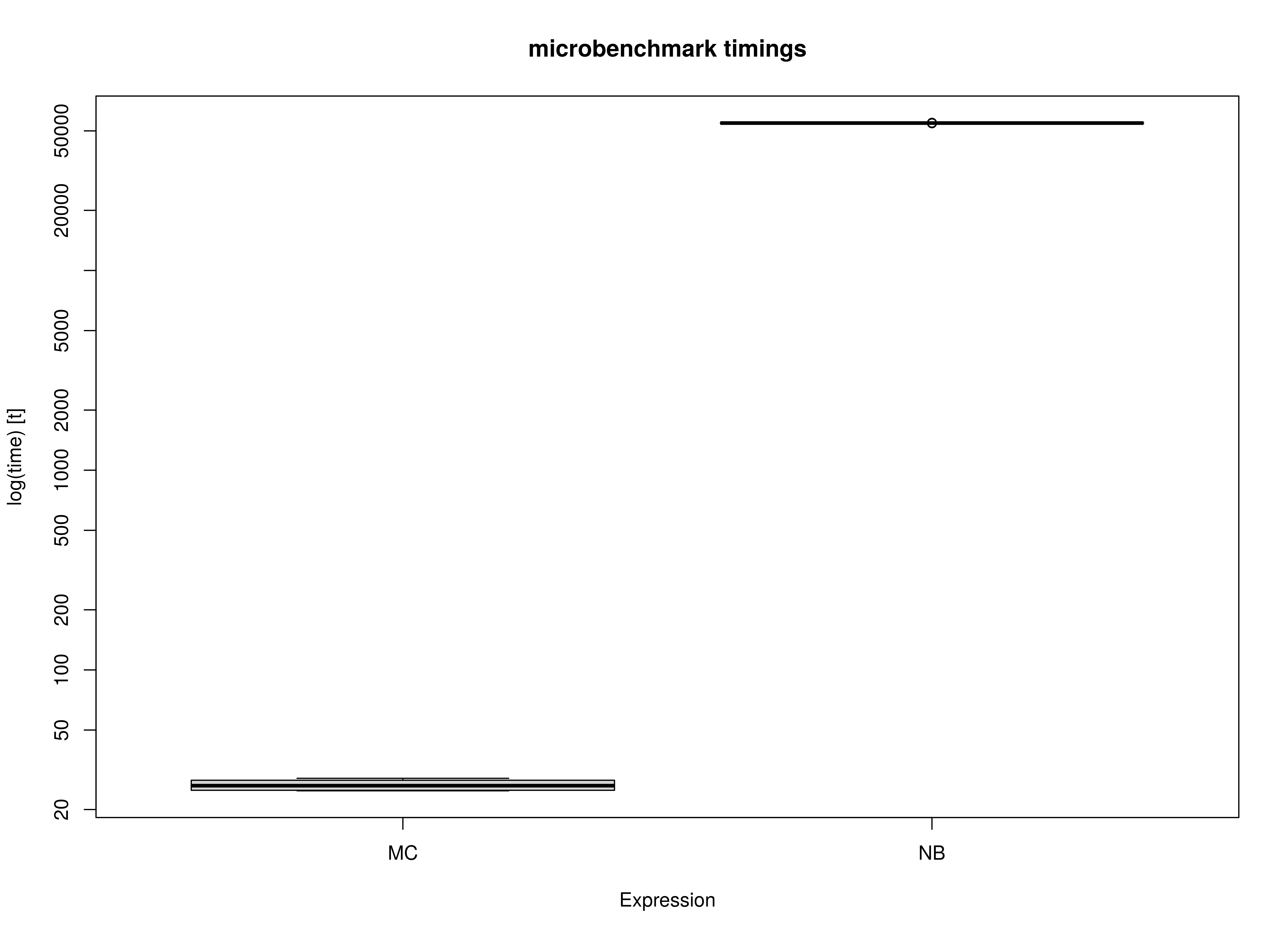
)Summary of Benchmark Results
summary(benchmark_fiml_01, unit = "ms")
#>   expr         min          lq        mean      median         uq         max
#> 1   MC    84.31734    86.23428    87.60209    86.83447    89.6138    92.56136
#> 2   NB 20772.68637 21129.81217 21260.76112 21225.07062 21535.4187 21682.53371
#>   neval
#> 1    10
#> 2    10
Summary of Benchmark Results Relative to the Faster Method
summary(benchmark_fiml_01, unit = "relative")
#>   expr      min      lq    mean   median       uq      max neval
#> 1   MC   1.0000   1.000   1.000   1.0000   1.0000   1.0000    10
#> 2   NB 246.3631 245.028 242.697 244.4314 240.3137 234.2504    10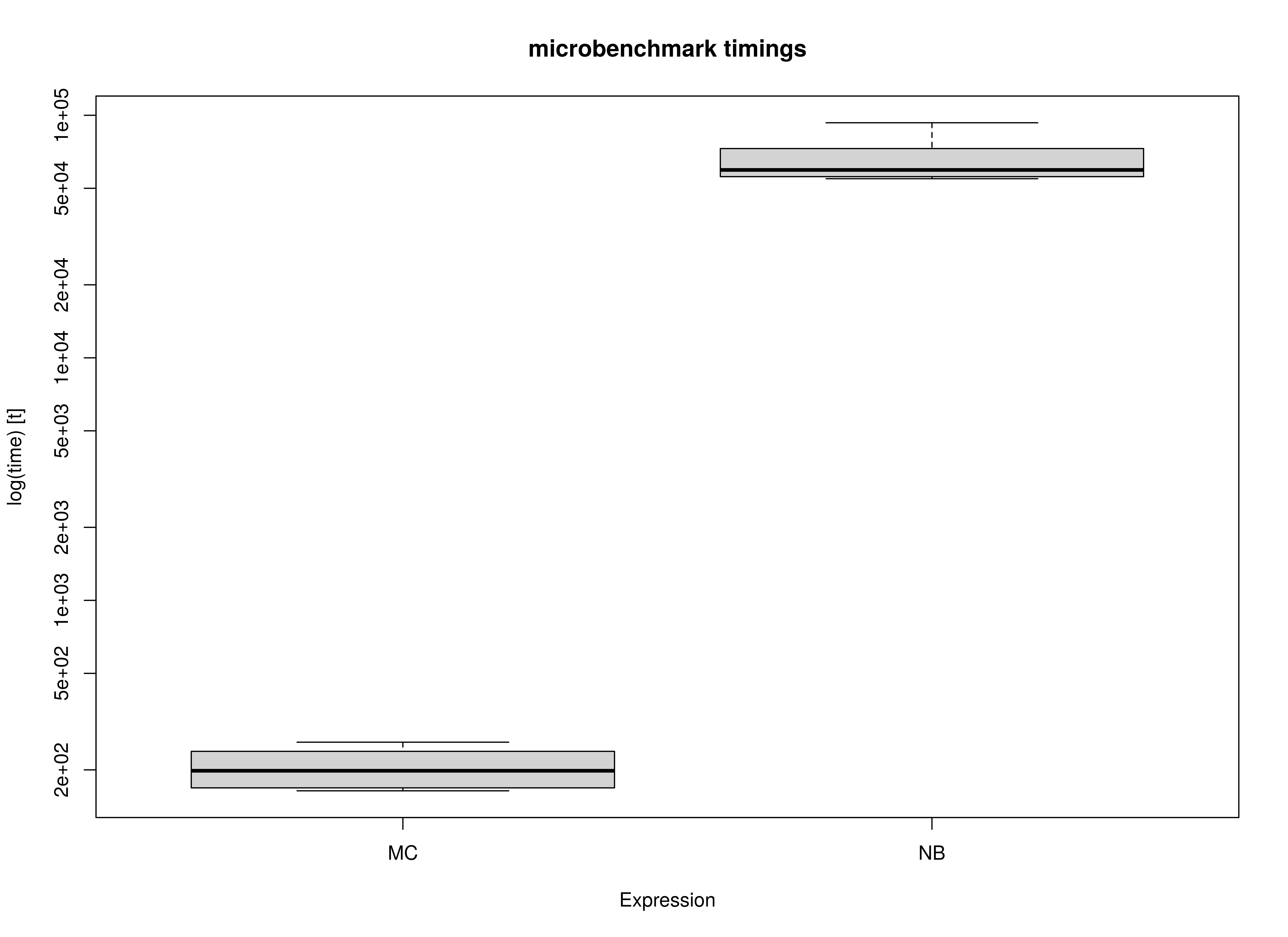
Benchmark - Monte Carlo Method with Precalculated Estimates
fit <- sem(
  data = df,
  model = model,
  missing = "fiml"
)
benchmark_fiml_02 <- microbenchmark(
  MC = MC(
    fit,
    R = R,
    decomposition = "chol",
    pd = FALSE
  ),
  NB = sem(
    data = df,
    model = model,
    missing = "fiml",
    se = "bootstrap",
    bootstrap = B
  ),
  times = 10
)
Summary of Benchmark Results
summary(benchmark_fiml_02, unit = "ms")
#>   expr         min        lq        mean     median          uq         max
#> 1   MC    16.69798    16.928    17.36761    16.9985    17.15756    18.98104
#> 2   NB 21060.47444 21333.220 21488.39948 21524.1889 21717.58101 21755.89528
#>   neval
#> 1    10
#> 2    10
Summary of Benchmark Results Relative to the Faster Method
summary(benchmark_fiml_02, unit = "relative")
#>   expr      min       lq     mean   median       uq      max neval
#> 1   MC    1.000    1.000    1.000    1.000    1.000    1.000    10
#> 2   NB 1261.259 1260.232 1237.268 1266.241 1265.773 1146.191    10