Benchmark: Comparing the Monte Carlo Method with Nonparametric Bootstrapping
Ivan Jacob Agaloos Pesigan
2026-06-13
Source:vignettes/benchmark-complete.Rmd
benchmark-complete.RmdWe compare the Monte Carlo (MC) method with nonparametric bootstrapping (NB) using the simple mediation model with complete data. One advantage of MC over NB is speed. This is because the model is only fitted once in MC whereas it is fitted many times in NB.
Model Specification
The indirect effect is defined by the product of the slopes of paths
X to M labeled as a and
M to Y labeled as b. In this
example, we are interested in the confidence intervals of
indirect defined as the product of a and
b using the := operator in the
lavaan model syntax.
model <- "
  Y ~ cp * X + b * M
  M ~ a * X
  X ~~ X
  indirect := a * b
  direct := cp
  total := cp + (a * b)
"
Model Fitting
We can now fit the model using the sem() function from
lavaan.
fit <- sem(data = df, model = model)Monte Carlo Confidence Intervals
The fit lavaan object can then be passed to
the MC() function from semmcci to generate
Monte Carlo confidence intervals.
MC(fit, R = 100L, alpha = 0.05)
#> Monte Carlo Confidence Intervals
#>             est     se   R   2.5%  97.5%
#> cp       0.2333 0.0296 100 0.1806 0.2903
#> b        0.5082 0.0279 100 0.4555 0.5527
#> a        0.4820 0.0280 100 0.4220 0.5301
#> X~~X     1.0590 0.0426 100 0.9751 1.1296
#> Y~~Y     0.5462 0.0231 100 0.5064 0.5959
#> M~~M     0.7527 0.0337 100 0.7024 0.8208
#> indirect 0.2449 0.0179 100 0.2058 0.2738
#> direct   0.2333 0.0296 100 0.1806 0.2903
#> total    0.4782 0.0295 100 0.4162 0.5283
Nonparametric Bootstrap Confidence Intervals
Nonparametric bootstrap confidence intervals can be generated in
lavaan using the following.
parameterEstimates(
  sem(
    data = df,
    model = model,
    se = "bootstrap",
    bootstrap = 100L
  )
)
#>        lhs op      rhs    label   est    se      z pvalue ci.lower ci.upper
#> 1        Y  ~        X       cp 0.233 0.025  9.395      0    0.183    0.278
#> 2        Y  ~        M        b 0.508 0.028 18.057      0    0.454    0.568
#> 3        M  ~        X        a 0.482 0.026 18.550      0    0.433    0.535
#> 4        X ~~        X          1.059 0.046 23.224      0    0.969    1.161
#> 5        Y ~~        Y          0.546 0.023 23.640      0    0.508    0.593
#> 6        M ~~        M          0.753 0.033 23.131      0    0.692    0.814
#> 7 indirect :=      a*b indirect 0.245 0.020 12.443      0    0.209    0.289
#> 8   direct :=       cp   direct 0.233 0.025  9.395      0    0.183    0.278
#> 9    total := cp+(a*b)    total 0.478 0.027 17.966      0    0.418    0.518
Benchmark
Arguments
| Variables | Values | Notes |
|---|---|---|
| R | 1000 | Number of Monte Carlo replications. |
| B | 1000 | Number of bootstrap samples. |
benchmark_complete_01 <- microbenchmark(
  MC = {
    fit <- sem(
      data = df,
      model = model
    )
    MC(
      fit,
      R = R,
      decomposition = "chol",
      pd = FALSE
    )
  },
  NB = sem(
    data = df,
    model = model,
    se = "bootstrap",
    bootstrap = B
  ),
  times = 10
)
Summary of Benchmark Results
summary(benchmark_complete_01, unit = "ms")
#>   expr        min          lq        mean      median          uq         max
#> 1   MC    55.0302    55.23845    58.02968    55.84808    58.06854    74.09966
#> 2   NB 10531.3588 10577.98131 10654.74758 10604.79738 10630.56465 10987.84880
#>   neval
#> 1    10
#> 2    10
Summary of Benchmark Results Relative to the Faster Method
summary(benchmark_complete_01, unit = "relative")
#>   expr      min       lq     mean   median       uq      max neval
#> 1   MC   1.0000   1.0000   1.0000   1.0000   1.0000   1.0000    10
#> 2   NB 191.3742 191.4967 183.6086 189.8865 183.0692 148.2847    10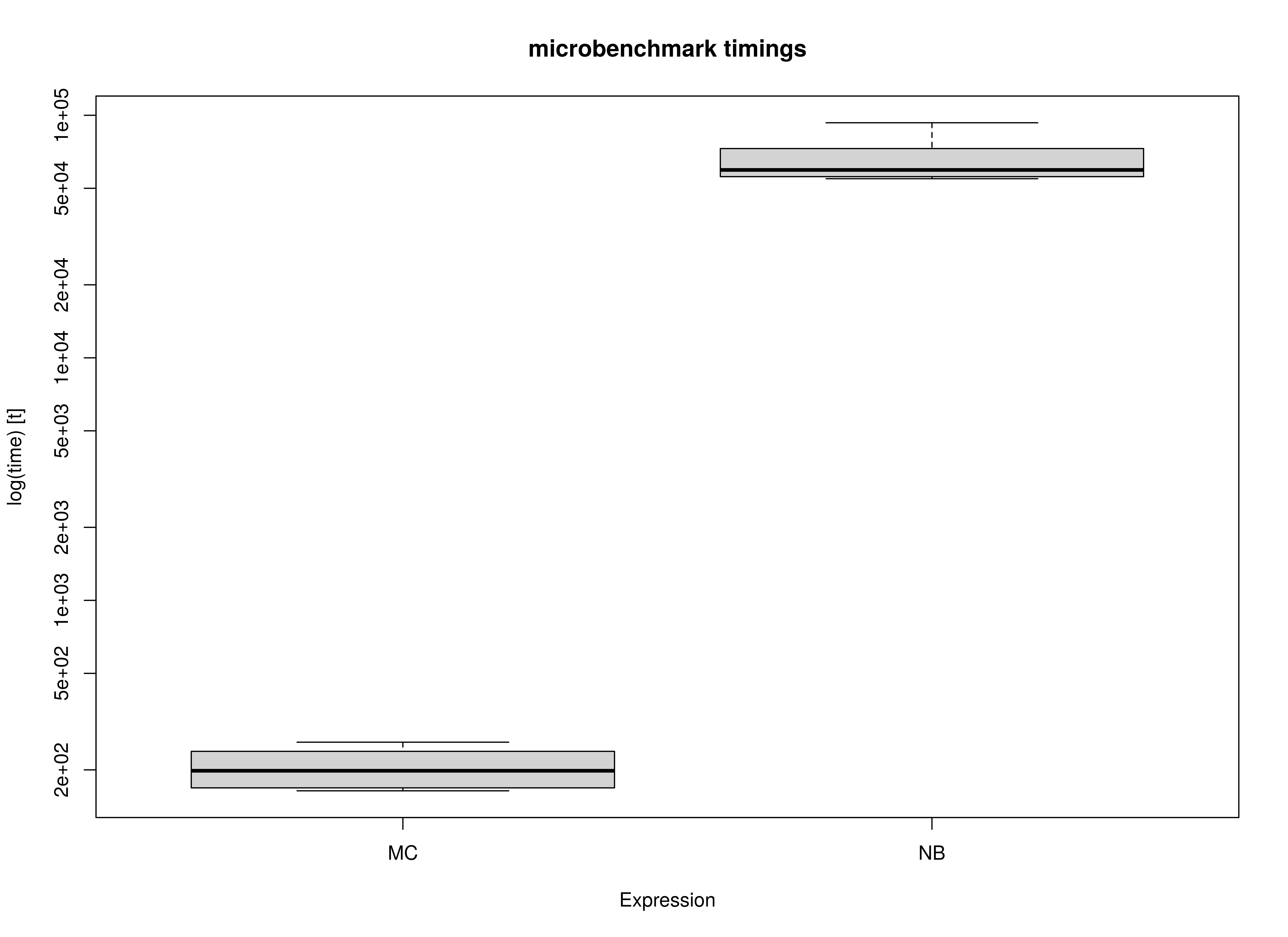
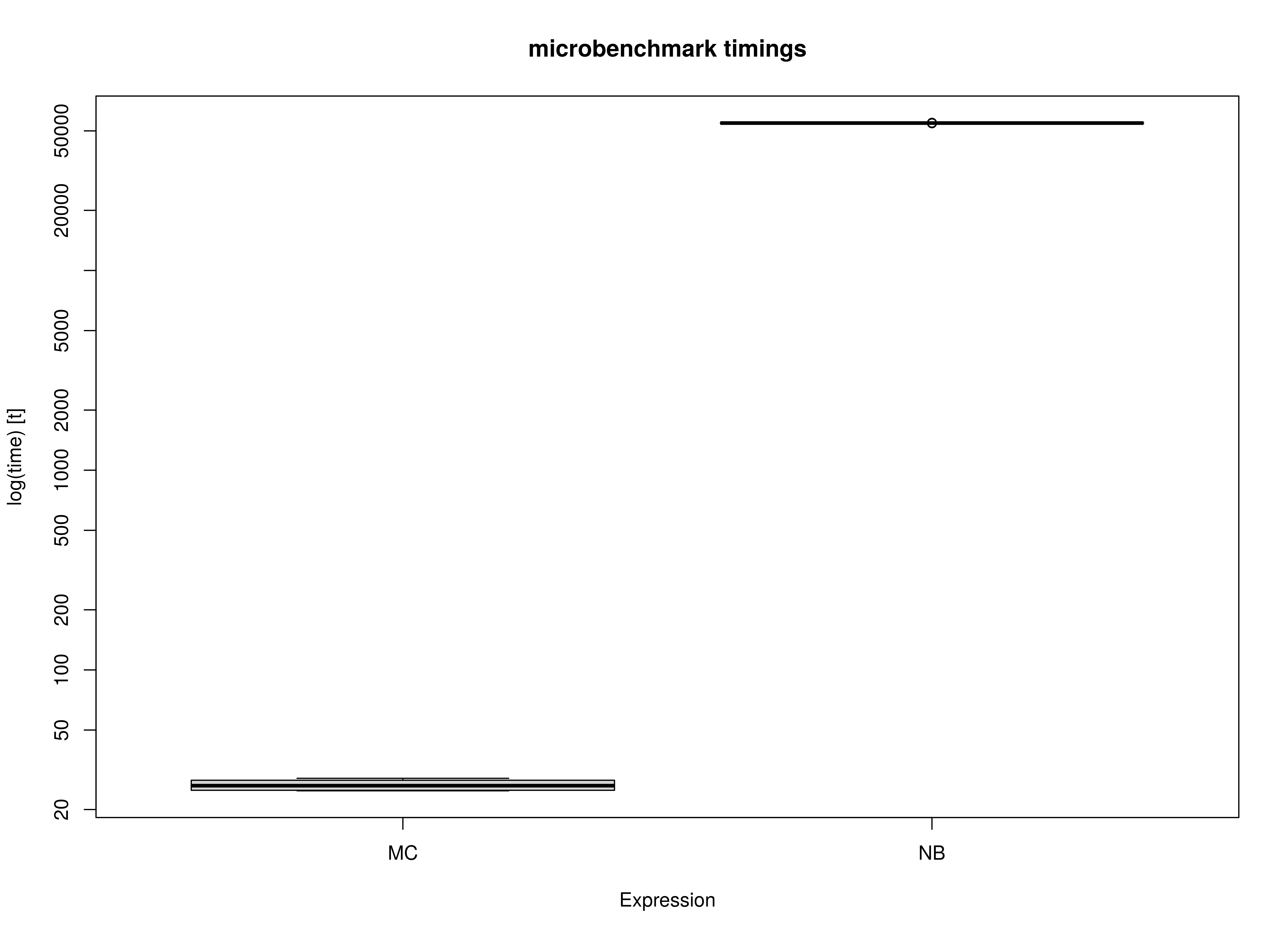
Benchmark - Monte Carlo Method with Precalculated Estimates
fit <- sem(
  data = df,
  model = model
)
benchmark_complete_02 <- microbenchmark(
  MC = MC(
    fit,
    R = R,
    decomposition = "chol",
    pd = FALSE
  ),
  NB = sem(
    data = df,
    model = model,
    se = "bootstrap",
    bootstrap = B
  ),
  times = 10
)
Summary of Benchmark Results
summary(benchmark_complete_02, unit = "ms")
#>   expr         min          lq        mean      median         uq         max
#> 1   MC    16.40516    16.70091    17.53686    16.73903    18.6218    20.88521
#> 2   NB 10341.15770 10374.74209 10584.52426 10633.36941 10753.5520 10814.98250
#>   neval
#> 1    10
#> 2    10
Summary of Benchmark Results Relative to the Faster Method
summary(benchmark_complete_02, unit = "relative")
#>   expr      min       lq     mean   median       uq      max neval
#> 1   MC   1.0000   1.0000   1.0000   1.0000   1.0000   1.0000    10
#> 2   NB 630.3601 621.2081 603.5585 635.2442 577.4711 517.8297    10