Multivariate Meta-Analysis of Discrete-Time VAR Estimates (Mixed-Effects Model)

Ivan Jacob Agaloos Pesigan

2024-08-12

Model

The measurement model is given by $$\begin{equation} \mathbf{y}_{i, t} = \boldsymbol{\eta}_{i, t} \end{equation}$$ where $\mathbf{y}_{i, t}$ represents a vector of observed variables and $\boldsymbol{\eta}_{i, t}$ a vector of latent variables for individual $i$ and time $t$. Since the observed and latent variables are equal, we only generate data from the dynamic structure.

The dynamic structure is given by $$\begin{equation} \boldsymbol{\eta}_{i, t} = \boldsymbol{\alpha} + \boldsymbol{\beta} \boldsymbol{\eta}_{i, t - 1} + \boldsymbol{\zeta}_{i, t}, \quad \mathrm{with} \quad \boldsymbol{\zeta}_{i, t} \sim \mathcal{N} \left( \mathbf{0}, \boldsymbol{\Psi} \right) \end{equation}$$ where $\boldsymbol{\eta}_{i, t}$, $\boldsymbol{\eta}_{i, t - 1}$, and $\boldsymbol{\zeta}_{i, t}$ are random variables, and $\boldsymbol{\alpha}$, $\boldsymbol{\beta}$, and $\boldsymbol{\Psi}$ are model parameters. Here, $\boldsymbol{\eta}_{i, t}$ is a vector of latent variables at time $t$ and individual $i$, $\boldsymbol{\eta}_{i, t - 1}$ represents a vector of latent variables at time $t - 1$ and individual $i$, and $\boldsymbol{\zeta}_{i, t}$ represents a vector of dynamic noise at time $t$ and individual $i$. $\boldsymbol{\alpha}$ denotes a vector of intercepts, $\boldsymbol{\beta}$ a matrix of autoregression and cross regression coefficients, and $\boldsymbol{\Psi}$ the covariance matrix of $\boldsymbol{\zeta}_{i, t}$.

An alternative representation of the dynamic noise is given by $$\begin{equation} \boldsymbol{\zeta}_{i, t} = \boldsymbol{\Psi}^{\frac{1}{2}} \mathbf{z}_{i, t}, \quad \mathrm{with} \quad \mathbf{z}_{i, t} \sim \mathcal{N} \left( \mathbf{0}, \mathbf{I} \right) \end{equation}$$ where $\left( \boldsymbol{\Psi}^{\frac{1}{2}} \right) \left( \boldsymbol{\Psi}^{\frac{1}{2}} \right)^{\prime} = \boldsymbol{\Psi}$ .

Data Generation

Notation

Let $t = 500$ be the number of time points and $n = 10$ be the number of individuals.

Let the initial condition $\boldsymbol{\eta}_{0}$ be given by

$$\begin{equation} \boldsymbol{\eta}_{0} \sim \mathcal{N} \left( \boldsymbol{\mu}_{\boldsymbol{\eta} \mid 0}, \boldsymbol{\Sigma}_{\boldsymbol{\eta} \mid 0} \right) \end{equation}$$

$$\begin{equation} \boldsymbol{\mu}_{\boldsymbol{\eta} \mid 0} = \left( \begin{array}{c} 0 \\ 0 \\ 0 \\ \end{array} \right) \end{equation}$$

$$\begin{equation} \boldsymbol{\Sigma}_{\boldsymbol{\eta} \mid 0} = \left( \begin{array}{ccc} 1 & 0 & 0 \\ 0 & 1 & 0 \\ 0 & 0 & 1 \\ \end{array} \right) . \end{equation}$$

Let the constant vector $\boldsymbol{\alpha}$ be given by

$$\begin{equation} \boldsymbol{\alpha} = \left( \begin{array}{c} 0 \\ 0 \\ 0 \\ \end{array} \right) . \end{equation}$$

Let the transition matrix $\boldsymbol{\beta}$ be normally distributed with the following means

$$\begin{equation} \left( \begin{array}{ccc} 0.7 & 0 & 0 \\ 0.5 & 0.6 & 0 \\ -0.1 & 0.4 & 0.5 \\ \end{array} \right) \end{equation}$$

and covariance matrix

$$\begin{equation} \left( \begin{array}{ccc} 0.01 & 0 & 0 & 0 & 0 & 0 & 0 & 0 & 0 \\ 0 & 0.01 & 0 & 0 & 0 & 0 & 0 & 0 & 0 \\ 0 & 0 & 0.01 & 0 & 0 & 0 & 0 & 0 & 0 \\ 0 & 0 & 0 & 0.01 & 0 & 0 & 0 & 0 & 0 \\ 0 & 0 & 0 & 0 & 0.01 & 0 & 0 & 0 & 0 \\ 0 & 0 & 0 & 0 & 0 & 0.01 & 0 & 0 & 0 \\ 0 & 0 & 0 & 0 & 0 & 0 & 0.01 & 0 & 0 \\ 0 & 0 & 0 & 0 & 0 & 0 & 0 & 0.01 & 0 \\ 0 & 0 & 0 & 0 & 0 & 0 & 0 & 0 & 0.01 \\ \end{array} \right) . \end{equation}$$

The SimBetaN function from the simStateSpace package generates random transition matrices from the multivariate normal distribution. Note that the function generates transition matrices that are weakly stationary.

Let the dynamic process noise $\boldsymbol{\Psi}$ be given by

$$\begin{equation} \boldsymbol{\Psi} = \left( \begin{array}{ccc} 0.1 & 0 & 0 \\ 0 & 0.1 & 0 \\ 0 & 0 & 0.1 \\ \end{array} \right) . \end{equation}$$

R Function Arguments

n
#> [1] 10
time
#> [1] 500
mu0
#> [[1]]
#> [1] 0 0 0
sigma0
#>      [,1] [,2] [,3]
#> [1,]    1    0    0
#> [2,]    0    1    0
#> [3,]    0    0    1
sigma0_l
#> [[1]]
#>      [,1] [,2] [,3]
#> [1,]    1    0    0
#> [2,]    0    1    0
#> [3,]    0    0    1
# first alpha in the list of length n
alpha[[1]]
#> [1] 0 0 0
# first beta in the list of length n
beta[[1]]
#>           [,1]       [,2]       [,3]
#> [1,] 0.6468498 0.02987347 0.09881764
#> [2,] 0.5821253 0.64048586 0.12907652
#> [3,] 0.1217450 0.33748281 0.46598132
psi
#>      [,1] [,2] [,3]
#> [1,]  0.1  0.0  0.0
#> [2,]  0.0  0.1  0.0
#> [3,]  0.0  0.0  0.1
psi_l
#> [[1]]
#>           [,1]      [,2]      [,3]
#> [1,] 0.3162278 0.0000000 0.0000000
#> [2,] 0.0000000 0.3162278 0.0000000
#> [3,] 0.0000000 0.0000000 0.3162278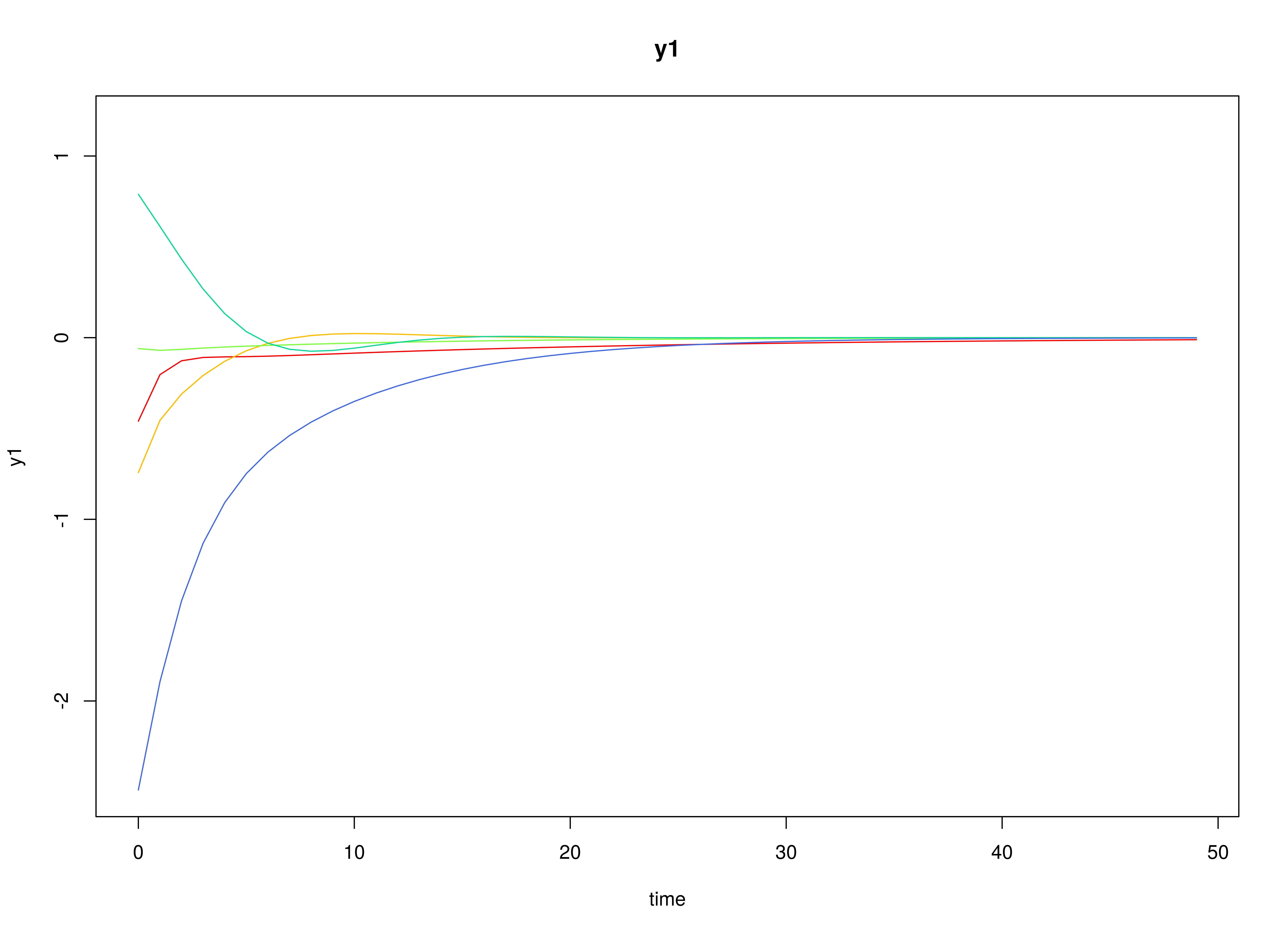

Visualizing the Dynamics Without Process Noise (n = 5 with Different Initial Condition)

Using the SimSSMVARIVary Function from the simStateSpace Package to Simulate Data

library(simStateSpace)
sim <- SimSSMVARIVary(
  n = n,
  time = time,
  mu0 = mu0,
  sigma0_l = sigma0_l,
  alpha = alpha,
  beta = beta,
  psi_l = psi_l
)
data <- as.data.frame(sim)
head(data)
#>   id time          y1         y2         y3
#> 1  1    0 -0.01667824  0.3471271 -0.5695179
#> 2  1    1  0.05129435  0.2859970 -0.2306270
#> 3  1    2 -0.33999076  0.6114834 -0.2472465
#> 4  1    3 -0.01661439 -0.2579420  0.2733639
#> 5  1    4 -0.50080900  0.2572493  0.1186636
#> 6  1    5 -0.19775105  0.1878050  0.3271472
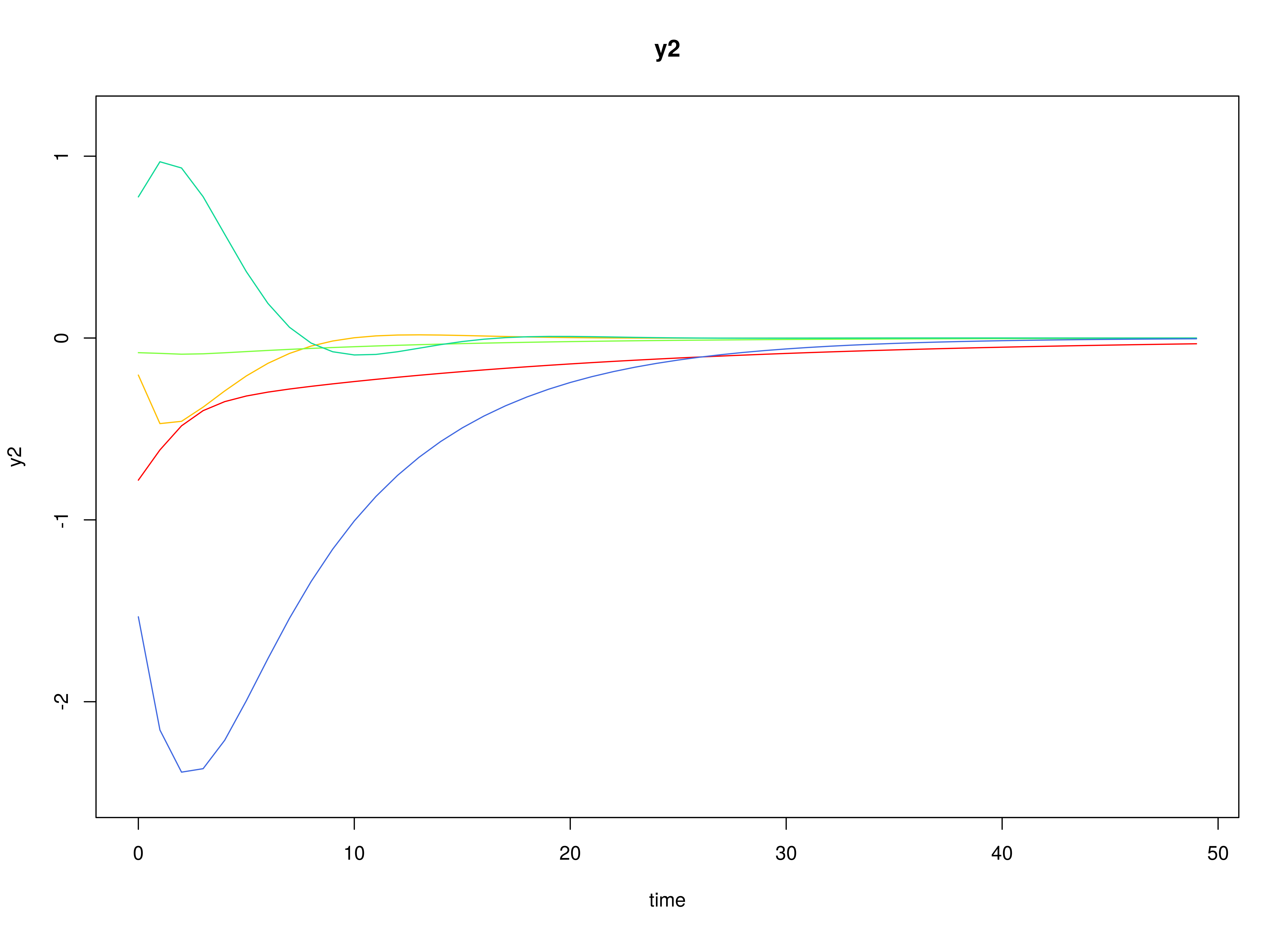
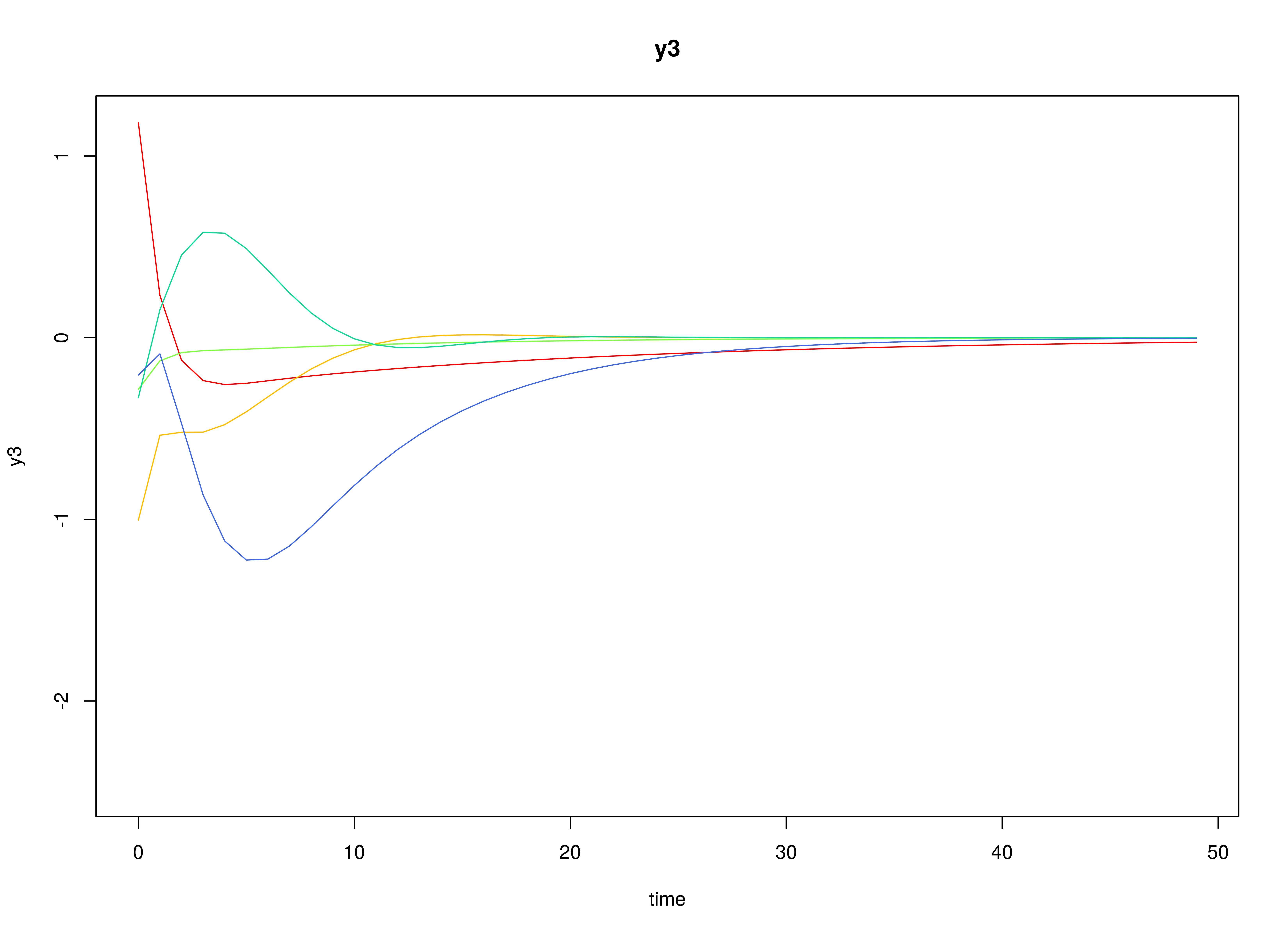
plot(sim)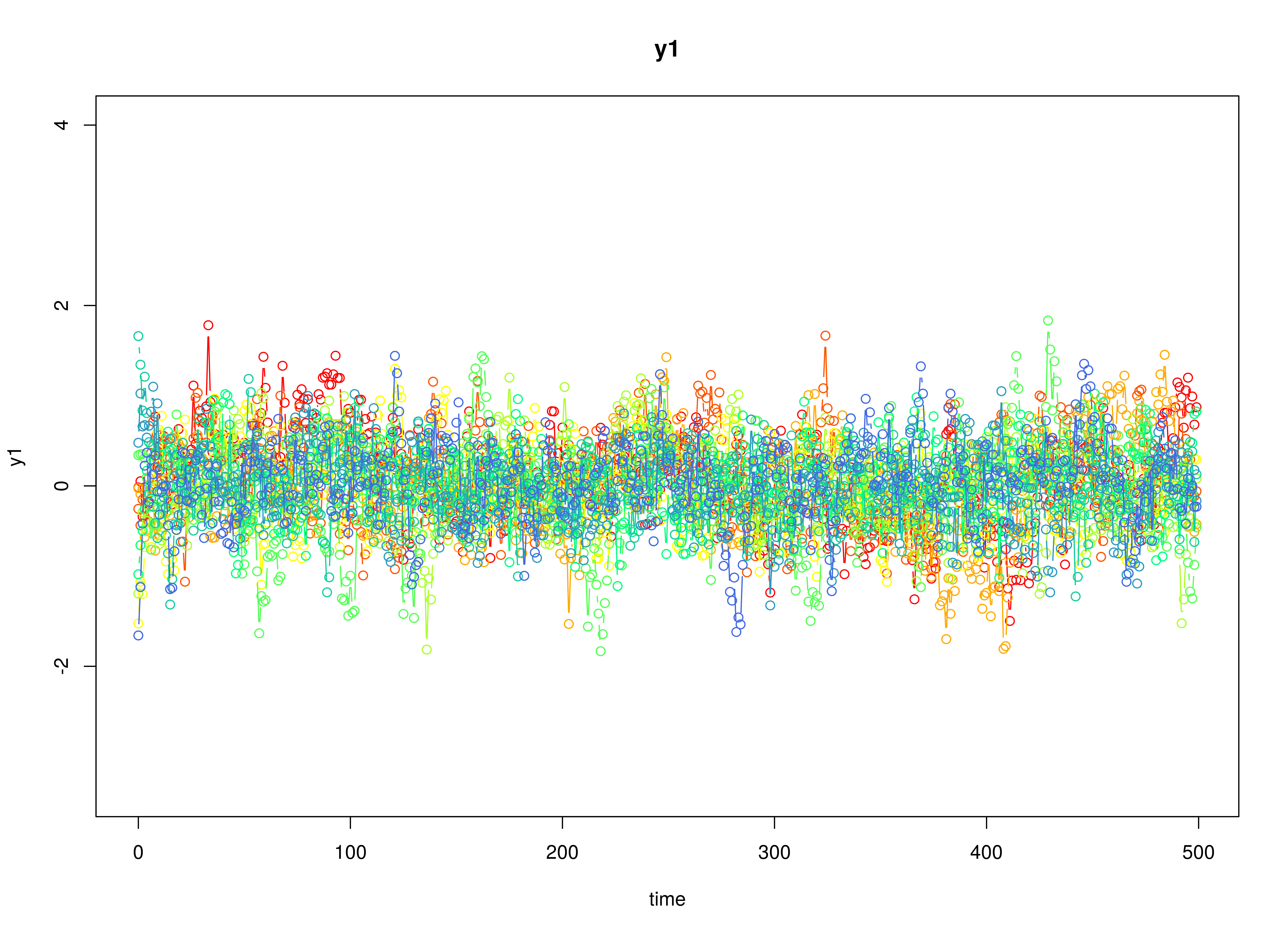

Model Fitting

The FitDTVARIDMx function fits a DT-VAR model on each individual $i$.

library(fitDTVARMx)
fit <- FitDTVARIDMx(
  data = data,
  observed = paste0("y", seq_len(k)),
  id = "id",
  ncores = parallel::detectCores()
)
fit
#> 
#> Means of the estimated paramaters per individual.
#>     beta_11     beta_21     beta_31     beta_12     beta_22     beta_32 
#>  0.65993097  0.50030159 -0.06447561  0.04378504  0.64014151  0.43853603 
#>     beta_13     beta_23     beta_33      psi_11      psi_22      psi_33 
#> -0.03958630  0.01326219  0.49408009  0.10016808  0.09849587  0.09896985

Multivariate Meta-Analysis

The MetaVARMx function performs multivariate meta-analysis using the estimated parameters and the corresponding sampling variance-covariance matrix for each individual $i$. Estimates with the prefix b0 correspond to the estimates of beta_mu. Estimates with the prefix b1 correspond to the estimates of the effects of x on y. Note that the effects of x on y in this case are all zeros. Estimates with the prefix t2 correspond to the estimates of beta_sigma. Estimates with the prefix i2 correspond to the estimates of heterogeniety.

x <- lapply(
  X = seq_len(n),
  FUN = function(i) {
    stats::rnorm(n = 2)
  }
)

library(metaVAR)
meta <- MetaVARMx(
  object = fit,
  x = x,
  ncores = parallel::detectCores()
)
#> Running Model with 72 parameters
#> 
#> Beginning initial fit attempt
#> Running Model with 72 parameters
#> 
#>  Lowest minimum so far:  -271.390852130041
#> 
#> Solution found

#> 
#>  Solution found!  Final fit=-271.39085 (started at 181.8219)  (1 attempt(s): 1 valid, 0 errors)
#>  Start values from best fit:
#> 0.657962241220472,0.51033967227259,-0.0567954629371411,0.0436811090007591,0.646664986578893,0.430527116896467,-0.0436390242964322,0.00154840596736853,0.487898856324546,-0.00171536960435824,-0.034191117183634,-0.0113769270104645,0.0127319728424718,-0.0508064711449298,0.0471040811841622,0.01281829562478,0.0546428473180705,0.00622674705947665,-0.0373278899849594,0.014326900038314,0.028172759926688,0.0243067434491325,-0.0599933548337579,0.0411649030024198,-0.00765519846664582,0.0184720225764948,-0.0429177873844594,0.0905260823187534,-0.021491827954899,-0.0684365870852203,-0.0385766717650605,-0.0397820953825144,0.0697830119273889,0.0216721203484656,0.00226476659139843,-0.0387608704309943,0.0938677998194565,0.0560340468885324,-0.00547507779064828,-0.0445965647751857,0.0122944202686715,0.0445209535326955,0.0226673510970409,-0.0177582479425677,0.0803964481064007,-0.00291115918767587,0.0339254072134867,-0.0558721012759551,0.00565473299932731,0.0491000139565992,0.0400736439582104,0.0423325753230253,-0.00259506146832299,0.0589777289459285,0.0182802588818472,0.0231307478025296,-0.0262048351748966,0.0434713659152594,-0.00220143633147934,0.0145752853266376,0.0178717992928919,-0.00739474262589907,0.0314365412417938,-0.0674172052618052,-0.0259762913278114,0.0297884215651565,1.06466555090781e-07,5.12114502520714e-08,-7.09828307697287e-08,1.54526931839517e-08,3.8067107662408e-09,2.2250738585072e-308
summary(meta)
#>            est     se       z      p    2.5%  97.5%
#> b0_1    0.6580 0.0318 20.6838 0.0000  0.5956 0.7203
#> b0_2    0.5103 0.0336 15.2090 0.0000  0.4446 0.5761
#> b0_3   -0.0568 0.0407 -1.3940 0.1633 -0.1366 0.0231
#> b0_4    0.0437 0.0211  2.0739 0.0381  0.0024 0.0850
#> b0_5    0.6467 0.0282 22.9417 0.0000  0.5914 0.7019
#> b0_6    0.4305 0.0379 11.3717 0.0000  0.3563 0.5047
#> b0_7   -0.0436 0.0300 -1.4533 0.1461 -0.1025 0.0152
#> b0_8    0.0015 0.0238  0.0649 0.9482 -0.0452 0.0483
#> b0_9    0.4879 0.0251 19.4167 0.0000  0.4386 0.5371
#> b1_11  -0.0017 0.0389 -0.0441 0.9648 -0.0779 0.0745
#> b1_21  -0.0342 0.0410 -0.8342 0.4042 -0.1145 0.0461
#> b1_31  -0.0114 0.0499 -0.2279 0.8197 -0.1092 0.0865
#> b1_41   0.0127 0.0264  0.4831 0.6291 -0.0389 0.0644
#> b1_51  -0.0508 0.0349 -1.4542 0.1459 -0.1193 0.0177
#> b1_61   0.0471 0.0468  1.0058 0.3145 -0.0447 0.1389
#> b1_71   0.0128 0.0367  0.3494 0.7268 -0.0591 0.0847
#> b1_81   0.0546 0.0290  1.8835 0.0596 -0.0022 0.1115
#> b1_91   0.0062 0.0306  0.2032 0.8390 -0.0538 0.0663
#> b1_12  -0.0373 0.0378 -0.9880 0.3232 -0.1114 0.0367
#> b1_22   0.0143 0.0398  0.3600 0.7188 -0.0637 0.0923
#> b1_32   0.0282 0.0484  0.5822 0.5605 -0.0667 0.1230
#> b1_42   0.0243 0.0253  0.9616 0.3362 -0.0252 0.0738
#> b1_52  -0.0600 0.0336 -1.7847 0.0743 -0.1259 0.0059
#> b1_62   0.0412 0.0451  0.9127 0.3614 -0.0472 0.1296
#> b1_72  -0.0077 0.0355 -0.2155 0.8294 -0.0773 0.0620
#> b1_82   0.0185 0.0281  0.6564 0.5116 -0.0367 0.0736
#> b1_92  -0.0429 0.0297 -1.4438 0.1488 -0.1012 0.0153
#> t2_1_1  0.0082 0.0042  1.9436 0.0519 -0.0001 0.0165
#> t2_2_1 -0.0019 0.0032 -0.6033 0.5463 -0.0083 0.0044
#> t2_3_1 -0.0062 0.0043 -1.4437 0.1488 -0.0146 0.0022
#> t2_4_1 -0.0035 0.0024 -1.4776 0.1395 -0.0081 0.0011
#> t2_5_1 -0.0036 0.0029 -1.2421 0.2142 -0.0093 0.0021
#> t2_6_1  0.0063 0.0041  1.5407 0.1234 -0.0017 0.0144
#> t2_7_1  0.0020 0.0029  0.6753 0.4995 -0.0037 0.0077
#> t2_8_1  0.0002 0.0022  0.0917 0.9269 -0.0042 0.0046
#> t2_9_1 -0.0035 0.0026 -1.3454 0.1785 -0.0086 0.0016
#> t2_2_2  0.0093 0.0047  1.9600 0.0500  0.0000 0.0185
#> t2_3_2  0.0067 0.0046  1.4726 0.1409 -0.0022 0.0157
#> t2_4_2  0.0003 0.0021  0.1502 0.8806 -0.0038 0.0044
#> t2_5_2 -0.0033 0.0030 -1.0939 0.2740 -0.0093 0.0026
#> t2_6_2 -0.0003 0.0038 -0.0916 0.9270 -0.0077 0.0071
#> t2_7_2  0.0037 0.0032  1.1559 0.2477 -0.0026 0.0100
#> t2_8_2  0.0021 0.0024  0.8500 0.3953 -0.0027 0.0069
#> t2_9_2 -0.0008 0.0025 -0.3330 0.7391 -0.0057 0.0041
#> t2_3_3  0.0143 0.0069  2.0667 0.0388  0.0007 0.0278
#> t2_4_3  0.0021 0.0026  0.8006 0.4234 -0.0030 0.0072
#> t2_5_3  0.0030 0.0035  0.8366 0.4028 -0.0040 0.0099
#> t2_6_3 -0.0086 0.0054 -1.5881 0.1123 -0.0192 0.0020
#> t2_7_3  0.0015 0.0037  0.4013 0.6882 -0.0057 0.0086
#> t2_8_3  0.0051 0.0033  1.5386 0.1239 -0.0014 0.0115
#> t2_9_3  0.0049 0.0034  1.4275 0.1534 -0.0018 0.0116
#> t2_4_4  0.0033 0.0019  1.7887 0.0737 -0.0003 0.0070
#> t2_5_4  0.0016 0.0018  0.8540 0.3931 -0.0020 0.0052
#> t2_6_4 -0.0001 0.0024 -0.0421 0.9664 -0.0048 0.0046
#> t2_7_4 -0.0003 0.0019 -0.1690 0.8658 -0.0041 0.0034
#> t2_8_4  0.0006 0.0015  0.4190 0.6752 -0.0023 0.0035
#> t2_9_4  0.0004 0.0016  0.2352 0.8140 -0.0027 0.0034
#> t2_5_5  0.0066 0.0033  1.9819 0.0475  0.0001 0.0132
#> t2_6_5 -0.0055 0.0036 -1.5134 0.1302 -0.0126 0.0016
#> t2_7_5 -0.0021 0.0026 -0.7974 0.4252 -0.0072 0.0030
#> t2_8_5  0.0013 0.0020  0.6483 0.5168 -0.0026 0.0052
#> t2_9_5  0.0034 0.0024  1.4621 0.1437 -0.0012 0.0081
#> t2_6_6  0.0126 0.0060  2.0893 0.0367  0.0008 0.0244
#> t2_7_6  0.0007 0.0034  0.1979 0.8431 -0.0060 0.0073
#> t2_8_6 -0.0018 0.0027 -0.6546 0.5127 -0.0072 0.0036
#> t2_9_6 -0.0058 0.0034 -1.6718 0.0946 -0.0125 0.0010
#> t2_7_7  0.0076 0.0038  1.9927 0.0463  0.0001 0.0150
#> t2_8_7  0.0038 0.0024  1.5453 0.1223 -0.0010 0.0086
#> t2_9_7 -0.0040 0.0026 -1.5527 0.1205 -0.0090 0.0010
#> t2_8_8  0.0045 0.0024  1.8871 0.0591 -0.0002 0.0091
#> t2_9_8  0.0000 0.0018 -0.0196 0.9843 -0.0035 0.0034
#> t2_9_9  0.0051 0.0027  1.9051 0.0568 -0.0001 0.0103
#> i2_1    0.8675 0.0591 14.6755 0.0000  0.7516 0.9833
#> i2_2    0.8814 0.0533 16.5374 0.0000  0.7770 0.9859
#> i2_3    0.9198 0.0357 25.7697 0.0000  0.8498 0.9898
#> i2_4    0.7956 0.0909  8.7485 0.0000  0.6173 0.9738
#> i2_5    0.8872 0.0505 17.5660 0.0000  0.7882 0.9862
#> i2_6    0.9371 0.0282 33.2267 0.0000  0.8818 0.9924
#> i2_7    0.8991 0.0455 19.7529 0.0000  0.8099 0.9883
#> i2_8    0.8430 0.0701 12.0223 0.0000  0.7055 0.9804
#> i2_9    0.8575 0.0642 13.3636 0.0000  0.7317 0.9832

References

Cheung, M. W.-L. (2015). Meta‐analysis: A structural equation modeling approach. Wiley. https://doi.org/10.1002/9781118957813

Hunter, M. D. (2017). State space modeling in an open source, modular, structural equation modeling environment. Structural Equation Modeling: A Multidisciplinary Journal, 25(2), 307–324. https://doi.org/10.1080/10705511.2017.1369354

Neale, M. C., Hunter, M. D., Pritikin, J. N., Zahery, M., Brick, T. R., Kirkpatrick, R. M., Estabrook, R., Bates, T. C., Maes, H. H., & Boker, S. M. (2015). OpenMx 2.0: Extended structural equation and statistical modeling. Psychometrika, 81(2), 535–549. https://doi.org/10.1007/s11336-014-9435-8

R Core Team. (2024). R: A language and environment for statistical computing. R Foundation for Statistical Computing. https://www.R-project.org/