Multivariate Meta-Analysis of Discrete-Time VAR Estimates (Fixed-Effect Model)

Ivan Jacob Agaloos Pesigan

2024-08-12

Model

The measurement model is given by $$\begin{equation} \mathbf{y}_{i, t} = \boldsymbol{\eta}_{i, t} \end{equation}$$ where $\mathbf{y}_{i, t}$ represents a vector of observed variables and $\boldsymbol{\eta}_{i, t}$ a vector of latent variables for individual $i$ and time $t$. Since the observed and latent variables are equal, we only generate data from the dynamic structure.

The dynamic structure is given by $$\begin{equation} \boldsymbol{\eta}_{i, t} = \boldsymbol{\alpha} + \boldsymbol{\beta} \boldsymbol{\eta}_{i, t - 1} + \boldsymbol{\zeta}_{i, t}, \quad \mathrm{with} \quad \boldsymbol{\zeta}_{i, t} \sim \mathcal{N} \left( \mathbf{0}, \boldsymbol{\Psi} \right) \end{equation}$$ where $\boldsymbol{\eta}_{i, t}$, $\boldsymbol{\eta}_{i, t - 1}$, and $\boldsymbol{\zeta}_{i, t}$ are random variables, and $\boldsymbol{\alpha}$, $\boldsymbol{\beta}$, and $\boldsymbol{\Psi}$ are model parameters. Here, $\boldsymbol{\eta}_{i, t}$ is a vector of latent variables at time $t$ and individual $i$, $\boldsymbol{\eta}_{i, t - 1}$ represents a vector of latent variables at time $t - 1$ and individual $i$, and $\boldsymbol{\zeta}_{i, t}$ represents a vector of dynamic noise at time $t$ and individual $i$. $\boldsymbol{\alpha}$ denotes a vector of intercepts, $\boldsymbol{\beta}$ a matrix of autoregression and cross regression coefficients, and $\boldsymbol{\Psi}$ the covariance matrix of $\boldsymbol{\zeta}_{i, t}$.

An alternative representation of the dynamic noise is given by $$\begin{equation} \boldsymbol{\zeta}_{i, t} = \boldsymbol{\Psi}^{\frac{1}{2}} \mathbf{z}_{i, t}, \quad \mathrm{with} \quad \mathbf{z}_{i, t} \sim \mathcal{N} \left( \mathbf{0}, \mathbf{I} \right) \end{equation}$$ where $\left( \boldsymbol{\Psi}^{\frac{1}{2}} \right) \left( \boldsymbol{\Psi}^{\frac{1}{2}} \right)^{\prime} = \boldsymbol{\Psi}$ .

Data Generation

Notation

Let $t = 500$ be the number of time points and $n = 10$ be the number of individuals.

Let the initial condition $\boldsymbol{\eta}_{0}$ be given by

$$\begin{equation} \boldsymbol{\eta}_{0} \sim \mathcal{N} \left( \boldsymbol{\mu}_{\boldsymbol{\eta} \mid 0}, \boldsymbol{\Sigma}_{\boldsymbol{\eta} \mid 0} \right) \end{equation}$$

$$\begin{equation} \boldsymbol{\mu}_{\boldsymbol{\eta} \mid 0} = \left( \begin{array}{c} 0 \\ 0 \\ 0 \\ \end{array} \right) \end{equation}$$

$$\begin{equation} \boldsymbol{\Sigma}_{\boldsymbol{\eta} \mid 0} = \left( \begin{array}{ccc} 1 & 0.2 & 0.2 \\ 0.2 & 1 & 0.2 \\ 0.2 & 0.2 & 1 \\ \end{array} \right) . \end{equation}$$

Let the constant vector $\boldsymbol{\alpha}$ be given by

$$\begin{equation} \boldsymbol{\alpha} = \left( \begin{array}{c} 0 \\ 0 \\ 0 \\ \end{array} \right) . \end{equation}$$

Let the transition matrix $\boldsymbol{\beta}$ be given by

$$\begin{equation} \boldsymbol{\beta} = \left( \begin{array}{ccc} 0.7 & 0 & 0 \\ 0.5 & 0.6 & 0 \\ -0.1 & 0.4 & 0.5 \\ \end{array} \right) . \end{equation}$$

Let the dynamic process noise $\boldsymbol{\Psi}$ be given by

$$\begin{equation} \boldsymbol{\Psi} = \left( \begin{array}{ccc} 0.1 & 0 & 0 \\ 0 & 0.1 & 0 \\ 0 & 0 & 0.1 \\ \end{array} \right) . \end{equation}$$

R Function Arguments

n
#> [1] 10
time
#> [1] 500
mu0
#> [1] 0 0 0
sigma0
#>      [,1] [,2] [,3]
#> [1,]  1.0  0.2  0.2
#> [2,]  0.2  1.0  0.2
#> [3,]  0.2  0.2  1.0
sigma0_l
#>      [,1]      [,2]      [,3]
#> [1,]  1.0 0.0000000 0.0000000
#> [2,]  0.2 0.9797959 0.0000000
#> [3,]  0.2 0.1632993 0.9660918
alpha
#> [1] 0 0 0
beta
#>      [,1] [,2] [,3]
#> [1,]  0.7  0.0  0.0
#> [2,]  0.5  0.6  0.0
#> [3,] -0.1  0.4  0.5
psi
#>      [,1] [,2] [,3]
#> [1,]  0.1  0.0  0.0
#> [2,]  0.0  0.1  0.0
#> [3,]  0.0  0.0  0.1
psi_l
#>           [,1]      [,2]      [,3]
#> [1,] 0.3162278 0.0000000 0.0000000
#> [2,] 0.0000000 0.3162278 0.0000000
#> [3,] 0.0000000 0.0000000 0.3162278

Visualizing the Dynamics Without Process Noise (n = 5 with Different Initial Condition)

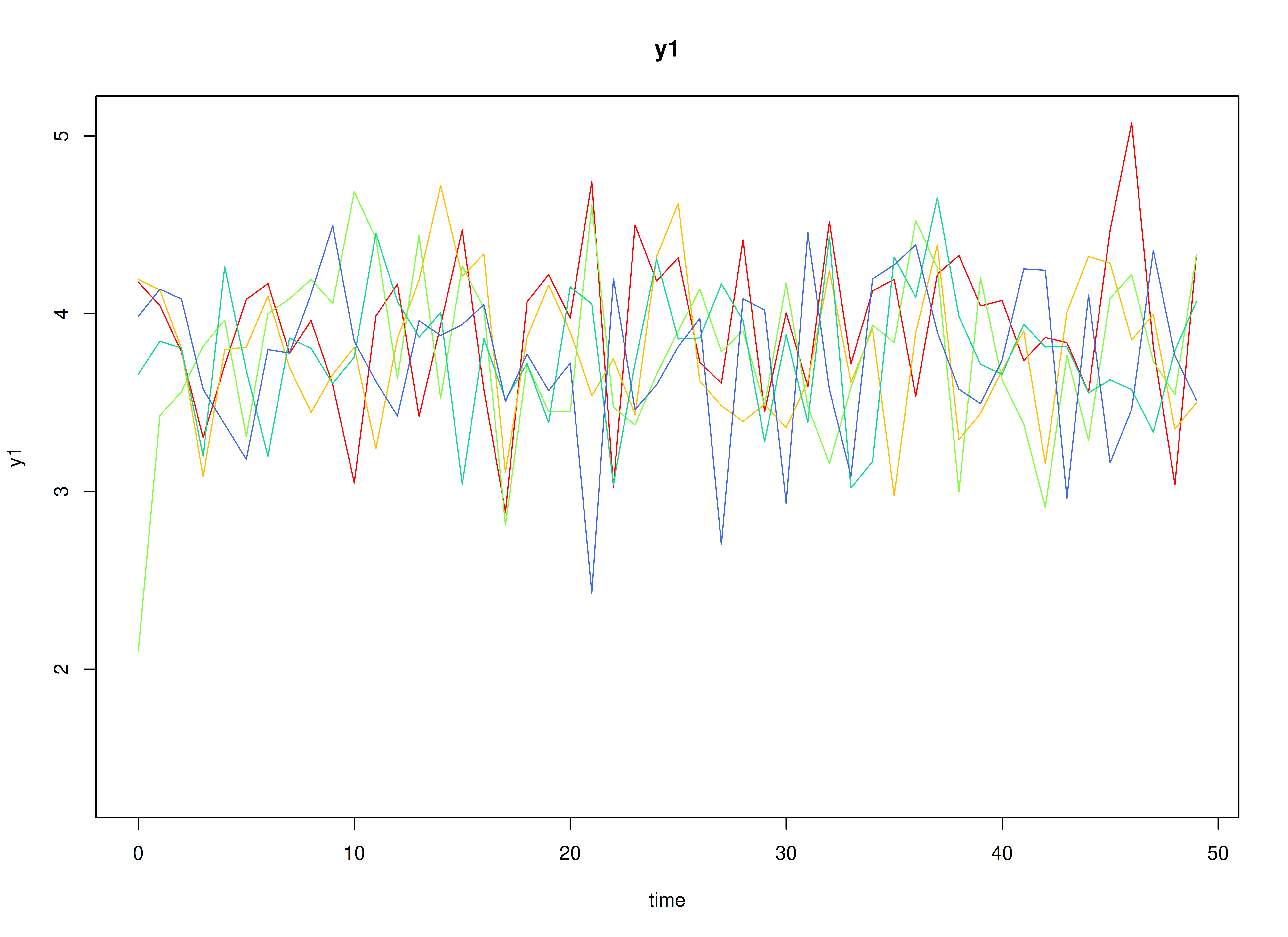
Using the SimSSMVARFixed Function from the simStateSpace Package to Simulate Data

library(simStateSpace)
sim <- SimSSMVARFixed(
  n = n,
  time = time,
  mu0 = mu0,
  sigma0_l = sigma0_l,
  alpha = alpha,
  beta = beta,
  psi_l = psi_l
)
data <- as.data.frame(sim)
head(data)
#>   id time          y1         y2         y3
#> 1  1    0 -1.84569501  0.5815402  0.8057225
#> 2  1    1 -1.34252674 -1.1219724  0.9873906
#> 3  1    2 -0.57123433 -1.1591679  0.1280274
#> 4  1    3 -0.44448720 -0.9783200 -0.3028425
#> 5  1    4 -0.28796224 -1.2222325 -0.3807219
#> 6  1    5  0.01622801 -1.2362032 -1.0056038
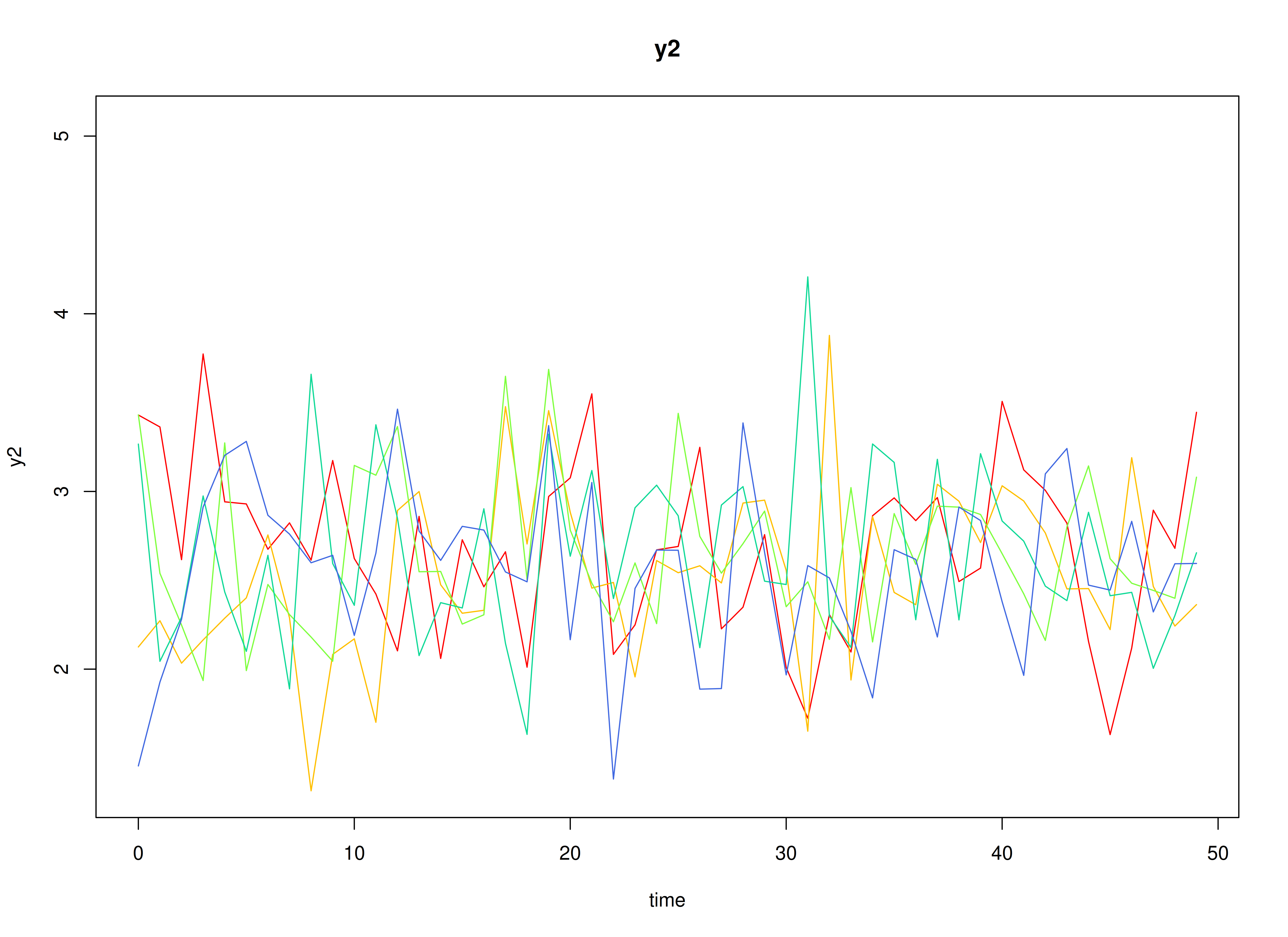
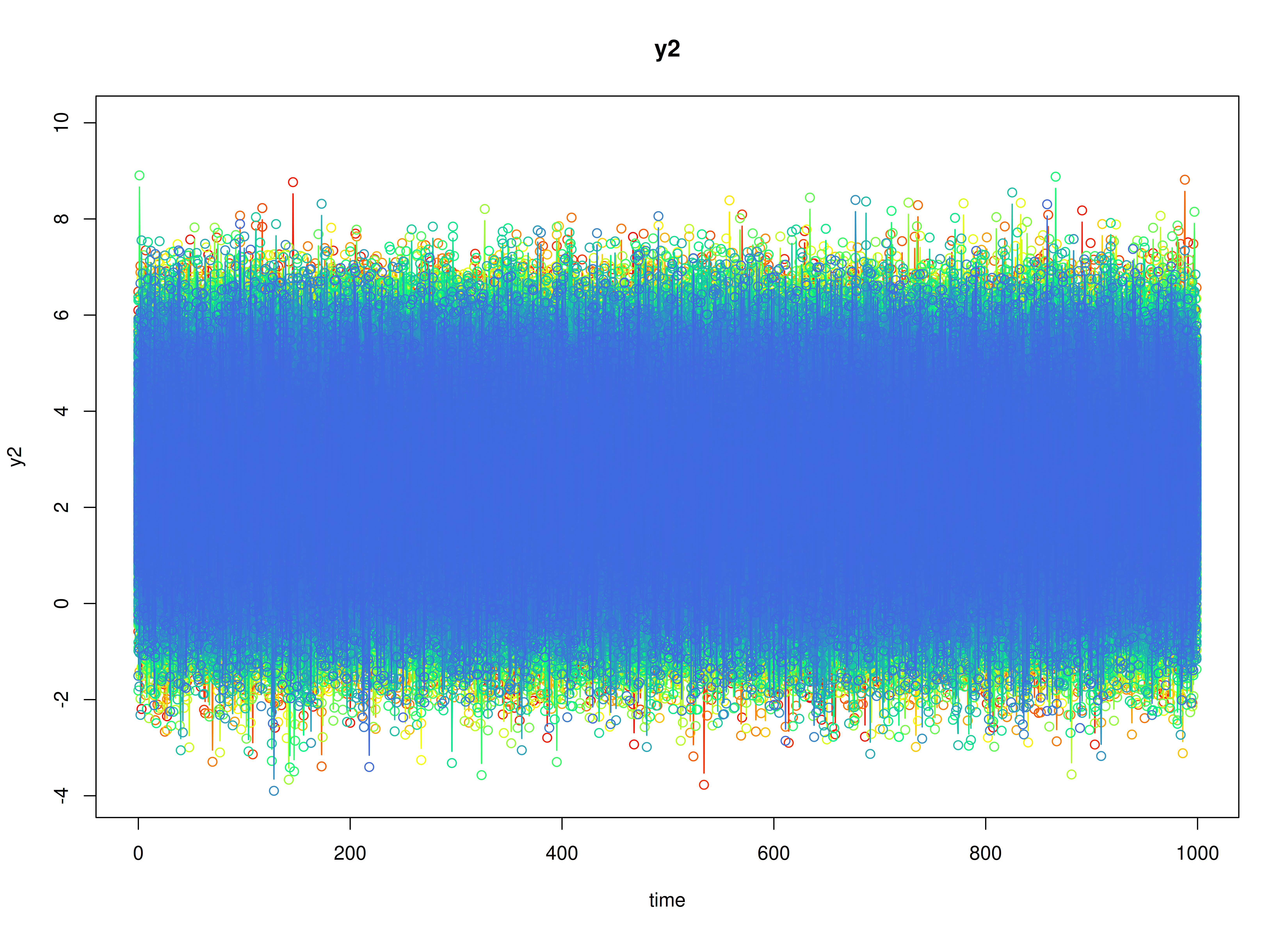
plot(sim)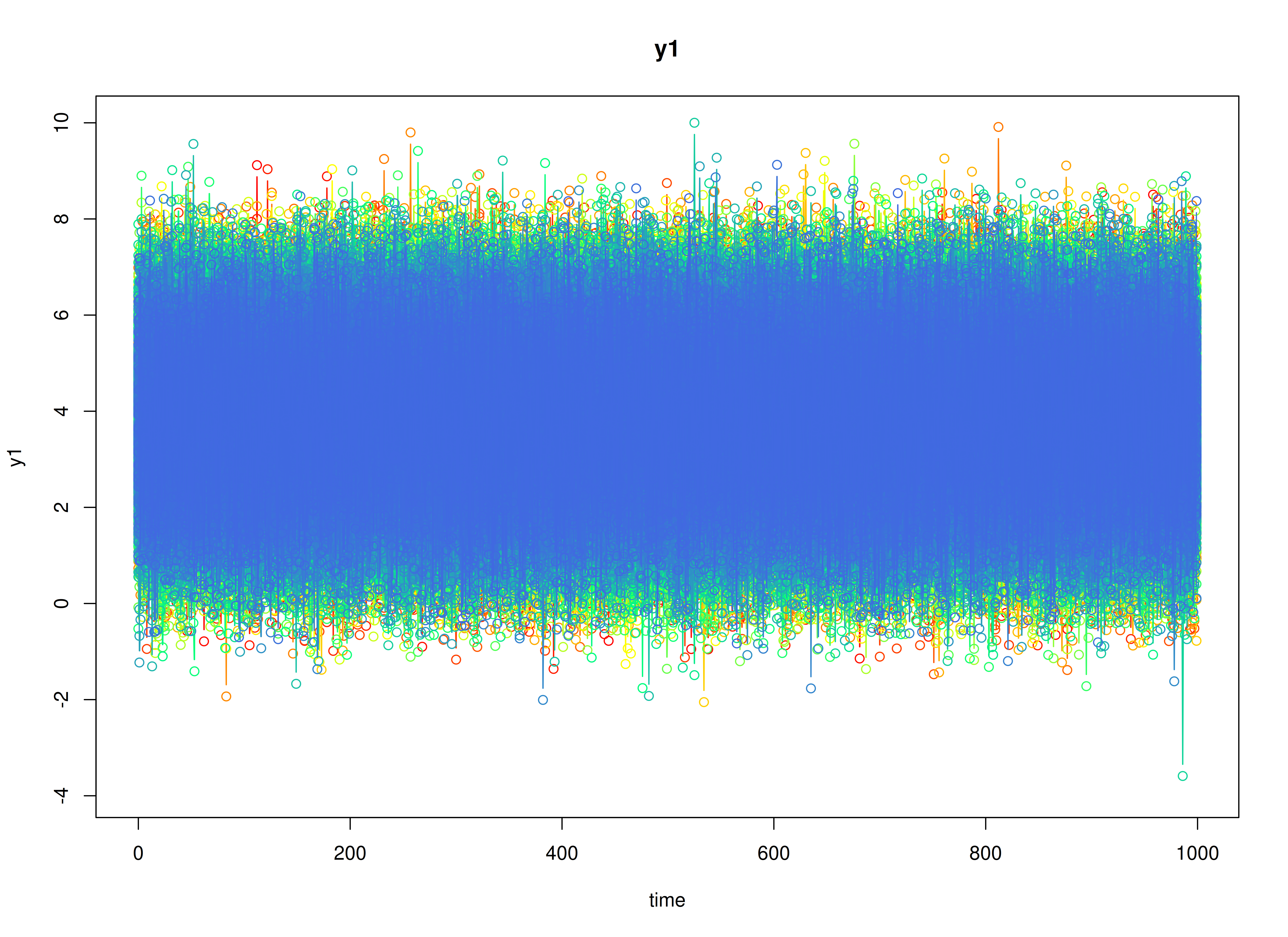

Model Fitting

The FitDTVARIDMx function fits a DT-VAR model on each individual $i$.

library(fitDTVARMx)
fit <- FitDTVARIDMx(
  data = data,
  observed = paste0("y", seq_len(k)),
  id = "id",
  ncores = parallel::detectCores()
)
fit
#> 
#> Means of the estimated paramaters per individual.
#>      beta_11      beta_21      beta_31      beta_12      beta_22      beta_32 
#>  0.689924482  0.486092103 -0.108580945  0.006642059  0.621491876  0.415330722 
#>      beta_13      beta_23      beta_33       psi_11       psi_22       psi_33 
#>  0.003199905 -0.015371495  0.499091854  0.098606259  0.099934823  0.099431124

Multivariate Meta-Analysis

The MetaVARMx function performs multivariate meta-analysis using the estimated parameters and the corresponding sampling variance-covariance matrix for each individual $i$. Estimates with the prefix b0 correspond to the estimates of beta.

library(metaVAR)
meta <- MetaVARMx(
  object = fit,
  random = FALSE,
  ncores = parallel::detectCores()
)
#> Running Model with 9 parameters
#> 
#> Beginning initial fit attempt
#> Running Model with 9 parameters
#> 
#>  Lowest minimum so far:  -374.744377237013
#> 
#> Solution found

#> 
#>  Solution found!  Final fit=-374.74438 (started at 25874.354)  (1 attempt(s): 1 valid, 0 errors)
#>  Start values from best fit:
#> 0.694366998609484,0.483106407790532,-0.108385418729956,0.00680176550454613,0.625084647828521,0.410742810401259,0.00183474121440079,-0.016822182670741,0.50097919233646
summary(meta)
#>          est     se       z      p    2.5%   97.5%
#> b0_1  0.6944 0.0111 62.3290 0.0000  0.6725  0.7162
#> b0_2  0.4831 0.0113 42.8908 0.0000  0.4610  0.5052
#> b0_3 -0.1084 0.0112 -9.6507 0.0000 -0.1304 -0.0864
#> b0_4  0.0068 0.0092  0.7383 0.4603 -0.0113  0.0249
#> b0_5  0.6251 0.0093 67.2811 0.0000  0.6069  0.6433
#> b0_6  0.4107 0.0093 44.1182 0.0000  0.3925  0.4290
#> b0_7  0.0018 0.0094  0.1950 0.8454 -0.0166  0.0203
#> b0_8 -0.0168 0.0095 -1.7740 0.0761 -0.0354  0.0018
#> b0_9  0.5010 0.0095 52.8912 0.0000  0.4824  0.5195

References

Cheung, M. W.-L. (2015). Meta‐analysis: A structural equation modeling approach. Wiley. https://doi.org/10.1002/9781118957813

Hunter, M. D. (2017). State space modeling in an open source, modular, structural equation modeling environment. Structural Equation Modeling: A Multidisciplinary Journal, 25(2), 307–324. https://doi.org/10.1080/10705511.2017.1369354

Neale, M. C., Hunter, M. D., Pritikin, J. N., Zahery, M., Brick, T. R., Kirkpatrick, R. M., Estabrook, R., Bates, T. C., Maes, H. H., & Boker, S. M. (2015). OpenMx 2.0: Extended structural equation and statistical modeling. Psychometrika, 81(2), 535–549. https://doi.org/10.1007/s11336-014-9435-8

R Core Team. (2024). R: A language and environment for statistical computing. R Foundation for Statistical Computing. https://www.R-project.org/