Multivariate Meta-Analysis of Continuous-Time VAR Estimates (Random-Effects Model)

Ivan Jacob Agaloos Pesigan

2024-08-12

Model

The measurement model is given by $$\begin{equation} \mathbf{y}_{i, t} = \boldsymbol{\nu} + \boldsymbol{\Lambda} \boldsymbol{\eta}_{i, t} + \boldsymbol{\varepsilon}_{i, t}, \quad \mathrm{with} \quad \boldsymbol{\varepsilon}_{i, t} \sim \mathcal{N} \left( \mathbf{0}, \boldsymbol{\Theta} \right) \end{equation}$$ where $\mathbf{y}_{i, t}$, $\boldsymbol{\eta}_{i, t}$, and $\boldsymbol{\varepsilon}_{i, t}$ are random variables and $\boldsymbol{\nu}$, $\boldsymbol{\Lambda}$, and $\boldsymbol{\Theta}$ are model parameters. $\mathbf{y}_{i, t}$ represents a vector of observed random variables, $\boldsymbol{\eta}_{i, t}$ a vector of latent random variables, and $\boldsymbol{\varepsilon}_{i, t}$ a vector of random measurement errors, at time $t$ and individual $i$. $\boldsymbol{\nu}$ denotes a vector of intercepts, $\boldsymbol{\Lambda}$ a matrix of factor loadings, and $\boldsymbol{\Theta}$ the covariance matrix of $\boldsymbol{\varepsilon}$.

An alternative representation of the measurement error is given by $$\begin{equation} \boldsymbol{\varepsilon}_{i, t} = \boldsymbol{\Theta}^{\frac{1}{2}} \mathbf{z}_{i, t}, \quad \mathrm{with} \quad \mathbf{z}_{i, t} \sim \mathcal{N} \left( \mathbf{0}, \mathbf{I} \right) \end{equation}$$ where $\mathbf{z}_{i, t}$ is a vector of independent standard normal random variables and $\left( \boldsymbol{\Theta}^{\frac{1}{2}} \right) \left( \boldsymbol{\Theta}^{\frac{1}{2}} \right)^{\prime} = \boldsymbol{\Theta}$ .

The dynamic structure is given by $$\begin{equation} \mathrm{d} \boldsymbol{\eta}_{i, t} = \boldsymbol{\Phi} \left( \boldsymbol{\eta}_{i, t} - \boldsymbol{\mu} \right) \mathrm{d}t + \boldsymbol{\Sigma}^{\frac{1}{2}} \mathrm{d} \mathbf{W}_{i, t} \end{equation}$$ where $\boldsymbol{\mu}$ is the long-term mean or equilibrium level, $\boldsymbol{\Phi}$ is the rate of mean reversion, determining how quickly the variable returns to its mean, $\boldsymbol{\Sigma}$ is the matrix of volatility or randomness in the process, and $\mathrm{d}\boldsymbol{W}$ is a Wiener process or Brownian motion, which represents random fluctuations.

Data Generation

Notation

Let $t = 500$ be the number of time points and $n = 10$ be the number of individuals.

Let the measurement model intecept vector $\boldsymbol{\nu}$ be given by

$$\begin{equation} \boldsymbol{\nu} = \left( \begin{array}{c} 0 \\ 0 \\ 0 \\ \end{array} \right) . \end{equation}$$

Let the factor loadings matrix $\boldsymbol{\Lambda}$ be given by

$$\begin{equation} \boldsymbol{\Lambda} = \left( \begin{array}{ccc} 1 & 0 & 0 \\ 0 & 1 & 0 \\ 0 & 0 & 1 \\ \end{array} \right) . \end{equation}$$

Let the measurement error covariance matrix $\boldsymbol{\Theta}$ be given by

$$\begin{equation} \boldsymbol{\Theta} = \left( \begin{array}{ccc} 0.2 & 0 & 0 \\ 0 & 0.2 & 0 \\ 0 & 0 & 0.2 \\ \end{array} \right) . \end{equation}$$

Let the initial condition $\boldsymbol{\eta}_{0}$ be given by

$$\begin{equation} \boldsymbol{\eta}_{0} \sim \mathcal{N} \left( \boldsymbol{\mu}_{\boldsymbol{\eta} \mid 0}, \boldsymbol{\Sigma}_{\boldsymbol{\eta} \mid 0} \right) \end{equation}$$

$$\begin{equation} \boldsymbol{\mu}_{\boldsymbol{\eta} \mid 0} = \left( \begin{array}{c} 0 \\ 0 \\ 0 \\ \end{array} \right) \end{equation}$$

$$\begin{equation} \boldsymbol{\Sigma}_{\boldsymbol{\eta} \mid 0} = \left( \begin{array}{ccc} 1 & 0 & 0 \\ 0 & 1 & 0 \\ 0 & 0 & 1 \\ \end{array} \right) . \end{equation}$$

Let the long-term mean vector $\boldsymbol{\mu}$ be given by

$$\begin{equation} \boldsymbol{\mu} = \left( \begin{array}{c} 0 \\ 0 \\ 0 \\ \end{array} \right) . \end{equation}$$

Let the drift matrix $\boldsymbol{\Phi}$ be normally distributed with the following means

$$\begin{equation} \left( \begin{array}{ccc} -0.357 & 0 & 0 \\ 0.771 & -0.511 & 0 \\ -0.45 & 0.729 & -0.693 \\ \end{array} \right) \end{equation}$$

and covariance matrix

$$\begin{equation} \left( \begin{array}{ccc} 0.01 & 0 & 0 & 0 & 0 & 0 & 0 & 0 & 0 \\ 0 & 0.01 & 0 & 0 & 0 & 0 & 0 & 0 & 0 \\ 0 & 0 & 0.01 & 0 & 0 & 0 & 0 & 0 & 0 \\ 0 & 0 & 0 & 0.01 & 0 & 0 & 0 & 0 & 0 \\ 0 & 0 & 0 & 0 & 0.01 & 0 & 0 & 0 & 0 \\ 0 & 0 & 0 & 0 & 0 & 0.01 & 0 & 0 & 0 \\ 0 & 0 & 0 & 0 & 0 & 0 & 0.01 & 0 & 0 \\ 0 & 0 & 0 & 0 & 0 & 0 & 0 & 0.01 & 0 \\ 0 & 0 & 0 & 0 & 0 & 0 & 0 & 0 & 0.01 \\ \end{array} \right) . \end{equation}$$

The SimPhiN function from the simStateSpace package generates random drift matrices from the multivariate normal distribution. Note that the function generates drift matrices that are stable.

Let the dynamic process noise covariance matrix $\boldsymbol{\Sigma}$ be given by

$$\begin{equation} \boldsymbol{\Sigma} = \left( \begin{array}{ccc} 0.1 & 0 & 0 \\ 0 & 0.1 & 0 \\ 0 & 0 & 0.1 \\ \end{array} \right) . \end{equation}$$

Let $\Delta t = 0.1$.

R Function Arguments

n
#> [1] 10
time
#> [1] 500
delta_t
#> [1] 0.1
mu0
#> [[1]]
#> [1] 0 0 0
sigma0
#>      [,1] [,2] [,3]
#> [1,]    1    0    0
#> [2,]    0    1    0
#> [3,]    0    0    1
sigma0_l
#> [[1]]
#>      [,1] [,2] [,3]
#> [1,]    1    0    0
#> [2,]    0    1    0
#> [3,]    0    0    1
mu
#> [[1]]
#> [1] 0 0 0
# first phi in the list of length n
phi[[1]]
#>            [,1]        [,2]        [,3]
#> [1,] -0.4101502  0.02987347  0.09881764
#> [2,]  0.8531253 -0.47051414  0.12907652
#> [3,] -0.2282550  0.66648281 -0.72701868
sigma
#>      [,1] [,2] [,3]
#> [1,]  0.1  0.0  0.0
#> [2,]  0.0  0.1  0.0
#> [3,]  0.0  0.0  0.1
sigma_l
#> [[1]]
#>           [,1]      [,2]      [,3]
#> [1,] 0.3162278 0.0000000 0.0000000
#> [2,] 0.0000000 0.3162278 0.0000000
#> [3,] 0.0000000 0.0000000 0.3162278
nu
#> [[1]]
#> [1] 0 0 0
lambda
#> [[1]]
#>      [,1] [,2] [,3]
#> [1,]    1    0    0
#> [2,]    0    1    0
#> [3,]    0    0    1
theta
#>      [,1] [,2] [,3]
#> [1,]  0.2  0.0  0.0
#> [2,]  0.0  0.2  0.0
#> [3,]  0.0  0.0  0.2
theta_l
#> [[1]]
#>           [,1]      [,2]      [,3]
#> [1,] 0.4472136 0.0000000 0.0000000
#> [2,] 0.0000000 0.4472136 0.0000000
#> [3,] 0.0000000 0.0000000 0.4472136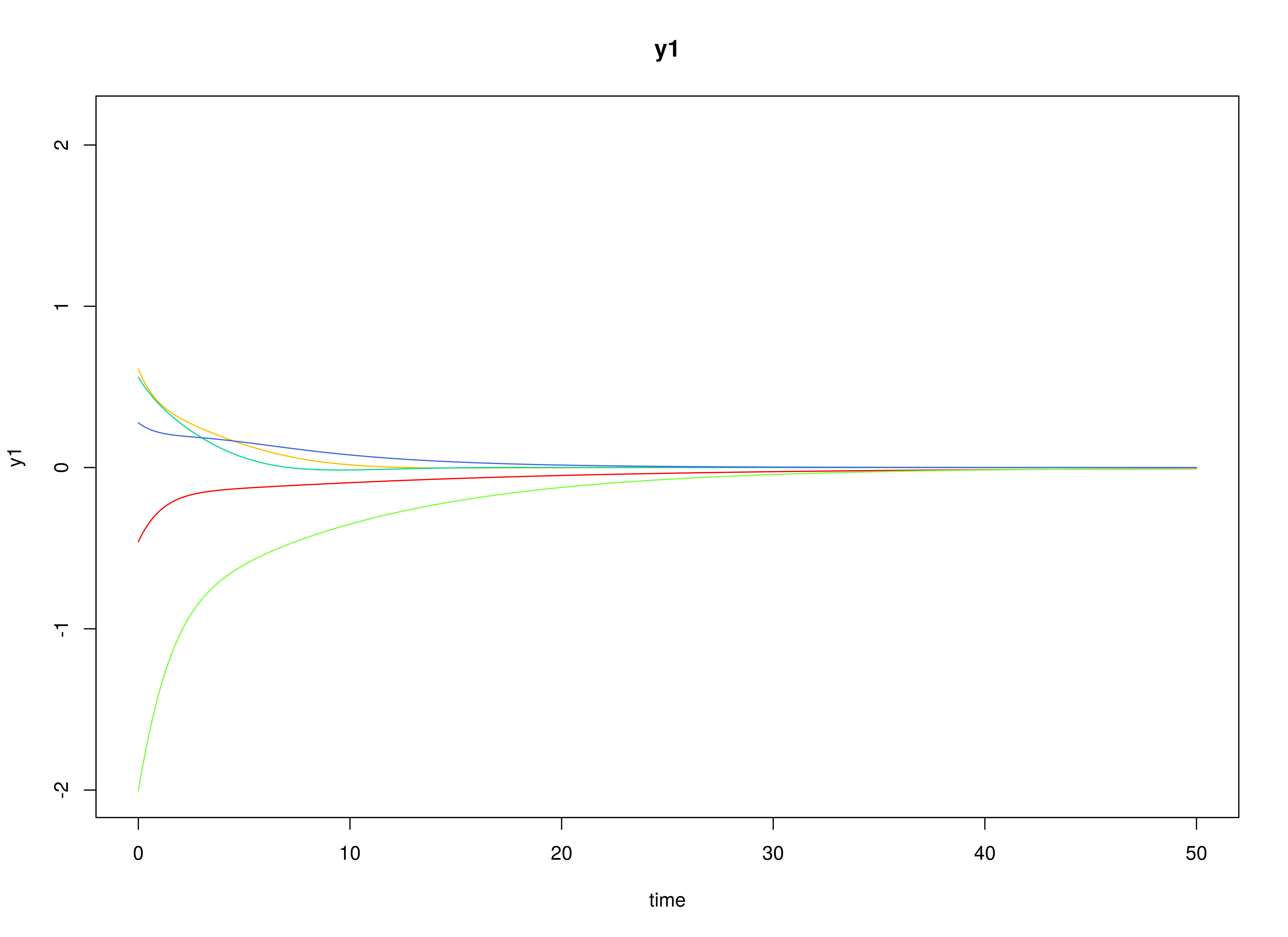

Visualizing the Dynamics Without Process Noise (n = 5 with Different Initial Condition)

Using the SimSSMOUIVary Function from the simStateSpace Package to Simulate Data

library(simStateSpace)
sim <- SimSSMOUIVary(
  n = n,
  time = time,
  delta_t = delta_t,
  mu0 = mu0,
  sigma0_l = sigma0_l,
  mu = mu,
  phi = phi,
  sigma_l = sigma_l,
  nu = nu,
  lambda = lambda,
  theta_l = theta_l
)
data <- as.data.frame(sim)
head(data)
#>   id time         y1         y2         y3
#> 1  1  0.0 -0.9066322  0.2077655 -0.1532395
#> 2  1  0.1 -2.0187881  0.1100828  1.5700524
#> 3  1  0.2 -1.9509792  0.7388884  0.6062416
#> 4  1  0.3 -0.7648885 -0.3710951  0.6992641
#> 5  1  0.4 -1.9989218 -1.4027964 -0.1971148
#> 6  1  0.5 -1.7412161 -0.2356327 -0.4460133
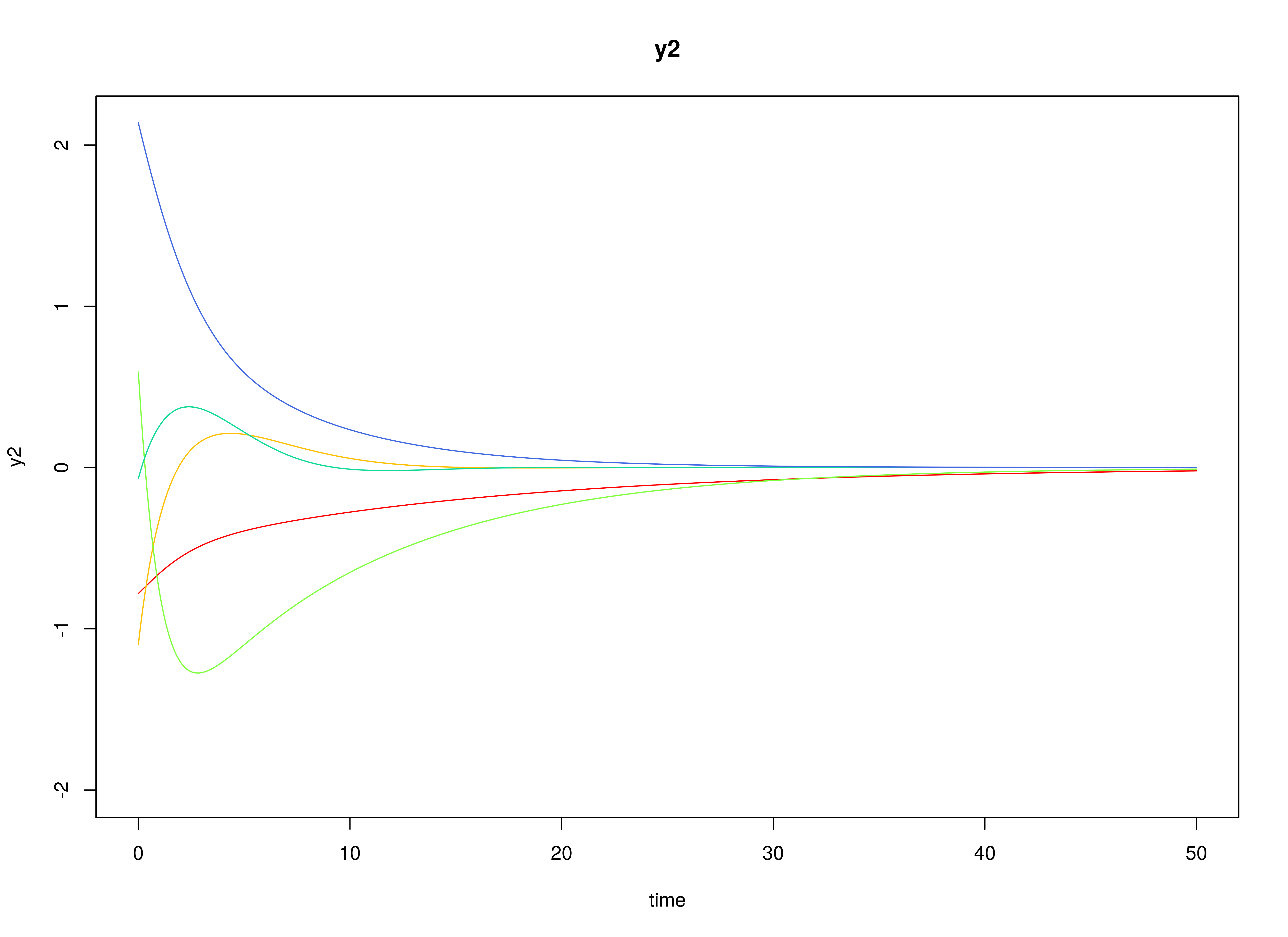
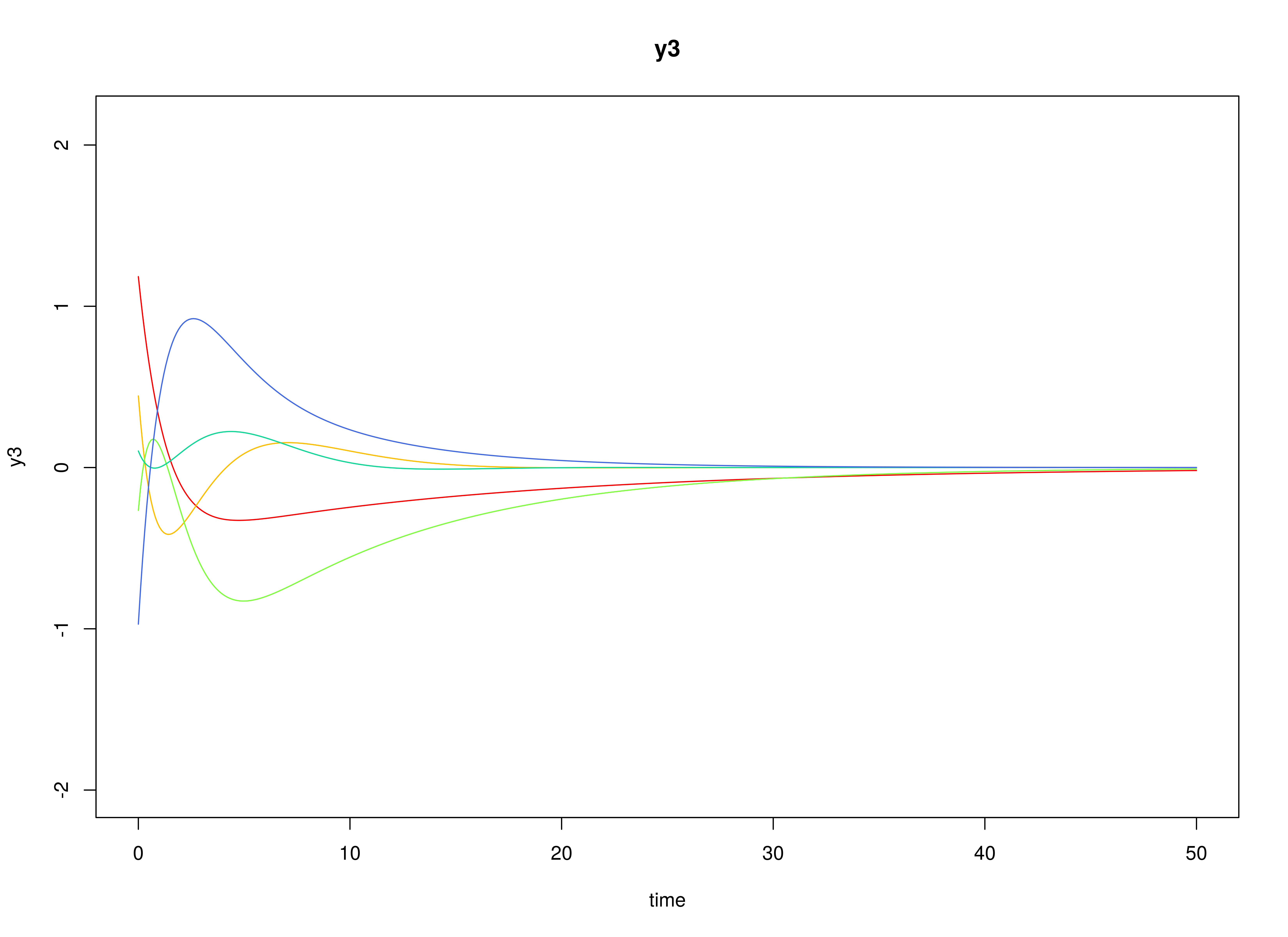
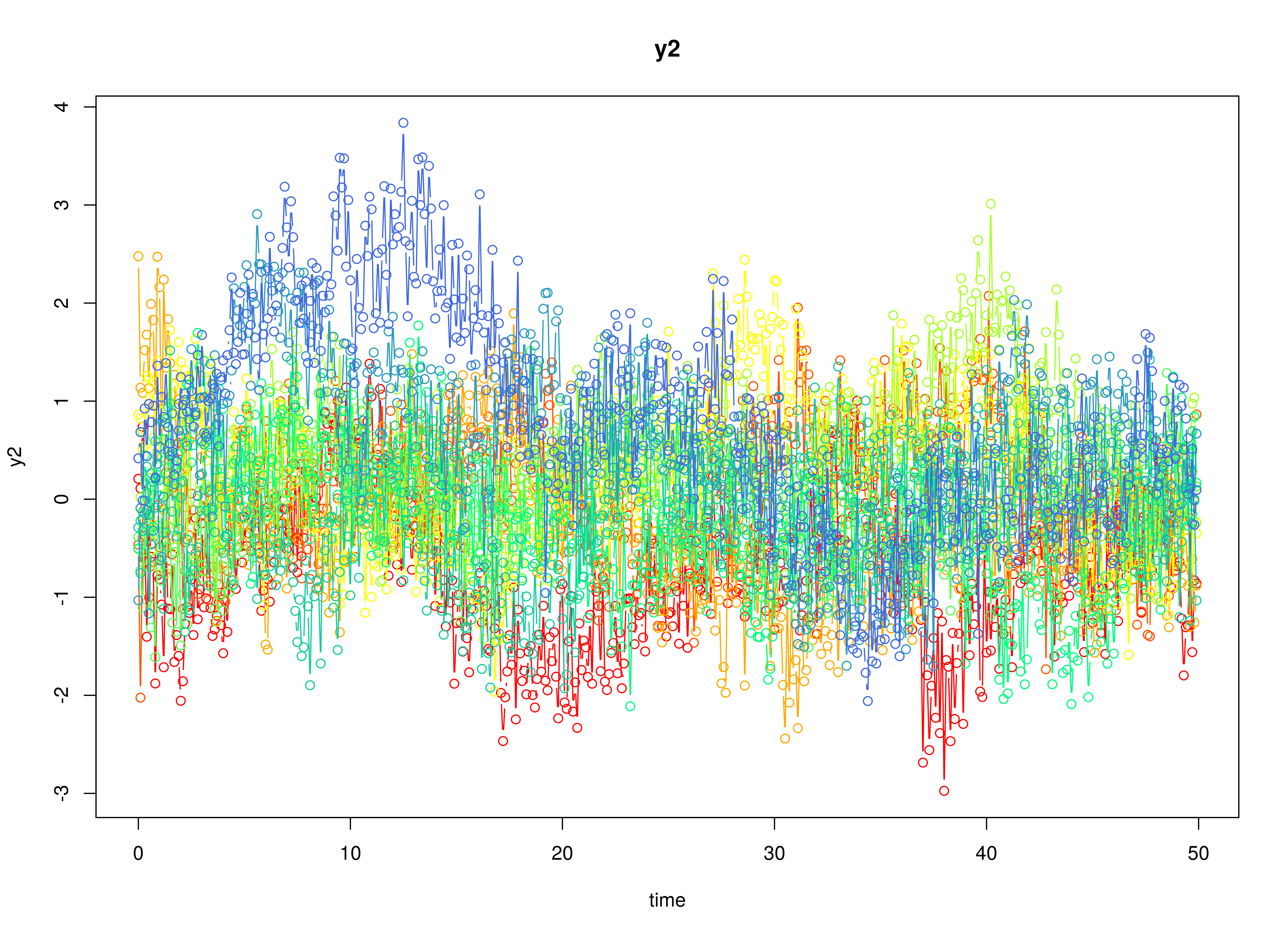
plot(sim)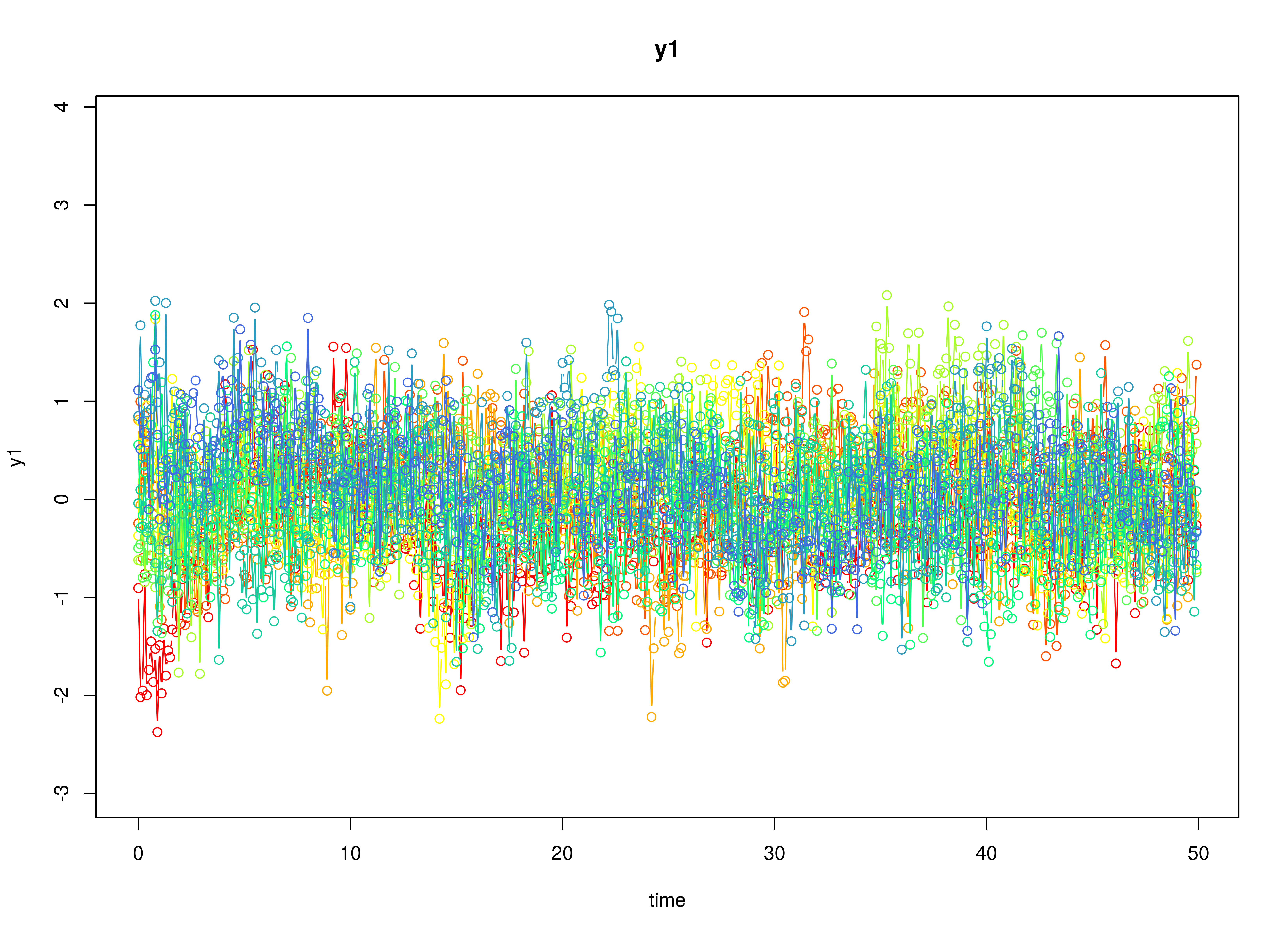

Model Fitting

The FitCTVARIDMx function fits a CT-VAR model on each individual $i$. The argument theta_fixed = FALSE is used here to model the measurement error variances.

library(fitCTVARMx)
fit <- FitCTVARIDMx(
  data = data,
  observed = paste0("y", seq_len(k)),
  id = "id",
  time = "time",
  theta_fixed = FALSE,
  ncores = parallel::detectCores()
)
fit
#> 
#> Means of the estimated paramaters per individual.
#>       phi_11       phi_21       phi_31       phi_12       phi_22       phi_32 
#> -0.329091189  0.851689092 -0.507551362  0.015917202 -0.509584686  1.032802799 
#>       phi_13       phi_23       phi_33     sigma_11     sigma_22     sigma_33 
#>  0.007716078  0.033385190 -1.017327464  0.100409860  0.101391404  0.121158245 
#>     theta_11     theta_22     theta_33 
#>  0.200496451  0.193508168  0.197870476

Multivariate Meta-Analysis

The MetaVARMx function performs multivariate meta-analysis using the estimated parameters and the corresponding sampling variance-covariance matrix for each individual $i$. Estimates with the prefix b0 correspond to the estimates of phi_mu. Estimates with the prefix t2 correspond to the estimates of phi_sigma. Estimates with the prefix i2 correspond to the estimates of heterogeniety.

library(metaVAR)
meta <- MetaVARMx(
  object = fit,
  ncores = parallel::detectCores()
)
#> Running Model with 54 parameters
#> 
#> Beginning initial fit attempt
#> Running Model with 54 parameters
#> 
#>  Lowest minimum so far:  -72.1152870564234
#>  Not all eigenvalues of the Hessian are positive: 17984.3584492803, 7823.59796373552, 6571.72627851725, 6462.11653985208, 6067.19867675505, 4750.99217992791, 4173.07515484696, 3471.88825206014, 3375.30072978953, 3372.38714546167, 3315.2214935166, 2901.23593545947, 2574.79043301278, 2245.06110562554, 1808.96773470412, 1447.72073791957, 1307.69968381221, 1267.94871105191, 1196.4977264325, 1005.38138197591, 964.01647961045, 940.875975445095, 936.74324688549, 882.365176005221, 757.191141604715, 738.295860861873, 603.244308892048, 592.72578907093, 542.406717249281, 532.477036577941, 494.665596989701, 457.243366583544, 424.840709062028, 375.227424147511, 294.503877402274, 246.544824091274, 224.420567786916, 222.948217078208, 215.202415132963, 212.493378626492, 207.681291751673, 186.995615323317, 180.388392682712, 154.154206760428, 115.480558579256, 96.2377924739206, 80.7414686660956, 71.975032928187, 36.9931497944026, 33.1865568534842, 19.7529698379684, 13.2586878148261, 11.4554671854342, -0.000649054145794033
#> 
#> Beginning fit attempt 1 of at maximum 1000 extra tries
#> Running Model with 54 parameters
#> 
#>  Lowest minimum so far:  -72.1152870564581
#>  Not all eigenvalues of the Hessian are positive: 17984.3617982683, 7823.59853904403, 6571.72615097289, 6462.11788935913, 6067.19418249775, 4750.98818207476, 4173.07386782431, 3471.88805836948, 3375.30096799724, 3372.38611414457, 3315.21883285237, 2901.23449834553, 2574.78998419306, 2245.05985031136, 1808.96882838259, 1447.72033436229, 1307.69998636733, 1267.94858548542, 1196.49799171926, 1005.38027054601, 964.014998076147, 940.875024594322, 936.741904838199, 882.364714952517, 757.191069780563, 738.296474397043, 603.244325555023, 592.726162044342, 542.407448716877, 532.477080785174, 494.665368564744, 457.243196486492, 424.841234731563, 375.228117164226, 294.504256015535, 246.545125705049, 224.421116038797, 222.949209133765, 215.202012710884, 212.493287078631, 207.681359411587, 186.995781904985, 180.388306501317, 154.154315789956, 115.480534643164, 96.2374328924389, 80.7417857927157, 71.9753634143554, 36.9931806956205, 33.1857618348157, 19.753422011944, 13.2578686116178, 11.4540920324459, -0.000878800997931927
#> 
#> Beginning fit attempt 2 of at maximum 1000 extra tries
#> Running Model with 54 parameters
#> 
#>  Lowest minimum so far:  -72.1152870564589
#> 
#> Solution found

#> 
#>  Solution found!  Final fit=-72.115287 (started at 207.37201)  (3 attempt(s): 3 valid, 0 errors)
#>  Start values from best fit:
#> -0.271000318612074,0.726425421703218,-0.310051774342087,-0.00696052901394403,-0.38185103546218,0.771686528655374,-0.000735443761825887,0.0236209135468562,-0.786740081734352,0.12032551183956,0.0784471494120775,-0.232226338142819,-0.129363333356534,-0.0497986099545828,0.11406280292163,0.0987300093287467,0.0190000541916716,-0.111344328222159,0.19340300983169,0.138062550078611,-0.0365720374993171,-0.0443667232655742,-0.106200277696935,0.0352035619070109,0.0898374314238645,0.127286761799942,2.13664182959341e-19,0.0248504492996431,-0.039872960444094,-0.066069264059006,-0.0365962924266653,0.00968109968191152,0.156787529656537,0.0124567294091376,-0.0199870314485065,-0.0331183924312503,-0.0183445422238564,0.00485282614669891,0.0785925375290673,3.86015210303806e-07,3.68335283961608e-07,7.28839204989482e-08,-1.91187106434466e-07,-1.02122447529622e-06,2.9202108783934e-08,4.40644987695317e-09,5.89599079840871e-09,-4.49020784537098e-08,1.3128799756775e-08,9.69415092301619e-09,-1.35442029197023e-08,1.39491360746515e-09,2.92816928453196e-09,6.94912332923949e-08
summary(meta)
#>            est     se       z      p    2.5%   97.5%
#> b0_1   -0.2710 0.1005 -2.6967 0.0070 -0.4680 -0.0740
#> b0_2    0.7264 0.1028  7.0682 0.0000  0.5250  0.9279
#> b0_3   -0.3101 0.1275 -2.4309 0.0151 -0.5600 -0.0601
#> b0_4   -0.0070 0.0881 -0.0790 0.9370 -0.1797  0.1658
#> b0_5   -0.3819 0.0796 -4.7998 0.0000 -0.5378 -0.2259
#> b0_6    0.7717 0.1154  6.6844 0.0000  0.5454  0.9980
#> b0_7   -0.0007 0.0737 -0.0100 0.9920 -0.1452  0.1437
#> b0_8    0.0236 0.0695  0.3398 0.7340 -0.1126  0.1598
#> b0_9   -0.7867 0.1296 -6.0707 0.0000 -1.0407 -0.5327
#> t2_1_1  0.0145 0.0240  0.6038 0.5460 -0.0325  0.0615
#> t2_2_1  0.0094 0.0247  0.3823 0.7023 -0.0390  0.0578
#> t2_3_1 -0.0279 0.0338 -0.8266 0.4085 -0.0942  0.0383
#> t2_4_1 -0.0156 0.0222 -0.7003 0.4838 -0.0591  0.0280
#> t2_5_1 -0.0060 0.0123 -0.4861 0.6269 -0.0302  0.0182
#> t2_6_1  0.0137 0.0228  0.6009 0.5479 -0.0310  0.0585
#> t2_7_1  0.0119 0.0172  0.6921 0.4889 -0.0218  0.0455
#> t2_8_1  0.0023 0.0122  0.1869 0.8517 -0.0217  0.0263
#> t2_9_1 -0.0134 0.0289 -0.4629 0.6434 -0.0701  0.0433
#> t2_2_2  0.0436 0.0389  1.1184 0.2634 -0.0328  0.1199
#> t2_3_2  0.0085 0.0343  0.2475 0.8045 -0.0587  0.0757
#> t2_4_2 -0.0172 0.0244 -0.7046 0.4811 -0.0651  0.0307
#> t2_5_2 -0.0125 0.0218 -0.5720 0.5673 -0.0553  0.0303
#> t2_6_2 -0.0116 0.0252 -0.4592 0.6461 -0.0611  0.0379
#> t2_7_2  0.0146 0.0189  0.7681 0.4424 -0.0226  0.0517
#> t2_8_2  0.0189 0.0199  0.9461 0.3441 -0.0202  0.0579
#> t2_9_2  0.0159 0.0302  0.5266 0.5984 -0.0432  0.0750
#> t2_3_3  0.0730 0.0604  1.2090 0.2267 -0.0453  0.1913
#> t2_4_3  0.0250 0.0302  0.8276 0.4079 -0.0342  0.0842
#> t2_5_3  0.0054 0.0214  0.2545 0.7991 -0.0364  0.0473
#> t2_6_3 -0.0412 0.0413 -0.9962 0.3192 -0.1221  0.0398
#> t2_7_3 -0.0181 0.0245 -0.7367 0.4613 -0.0661  0.0300
#> t2_8_3  0.0080 0.0191  0.4176 0.6763 -0.0295  0.0455
#> t2_9_3  0.0434 0.0474  0.9157 0.3598 -0.0495  0.1364
#> t2_4_4  0.0188 0.0234  0.8037 0.4216 -0.0271  0.0648
#> t2_5_4  0.0068 0.0132  0.5185 0.6041 -0.0190  0.0326
#> t2_6_4 -0.0129 0.0226 -0.5717 0.5675 -0.0572  0.0314
#> t2_7_4 -0.0152 0.0189 -0.8025 0.4222 -0.0523  0.0219
#> t2_8_4 -0.0054 0.0125 -0.4353 0.6633 -0.0299  0.0191
#> t2_9_4  0.0146 0.0283  0.5170 0.6052 -0.0408  0.0701
#> t2_5_5  0.0064 0.0119  0.5417 0.5881 -0.0169  0.0297
#> t2_6_5  0.0023 0.0148  0.1571 0.8751 -0.0267  0.0314
#> t2_7_5 -0.0047 0.0107 -0.4353 0.6634 -0.0256  0.0163
#> t2_8_5 -0.0054 0.0111 -0.4865 0.6266 -0.0272  0.0164
#> t2_9_5 -0.0079 0.0199 -0.3991 0.6898 -0.0468  0.0310
#> t2_6_6  0.0298 0.0342  0.8691 0.3848 -0.0373  0.0968
#> t2_7_6  0.0105 0.0195  0.5399 0.5892 -0.0277  0.0488
#> t2_8_6 -0.0082 0.0144 -0.5665 0.5711 -0.0365  0.0201
#> t2_9_6 -0.0392 0.0447 -0.8773 0.3803 -0.1267  0.0484
#> t2_7_7  0.0127 0.0164  0.7698 0.4414 -0.0196  0.0449
#> t2_8_7  0.0046 0.0101  0.4547 0.6494 -0.0152  0.0244
#> t2_9_7 -0.0137 0.0256 -0.5355 0.5923 -0.0638  0.0364
#> t2_8_8  0.0085 0.0114  0.7480 0.4545 -0.0139  0.0310
#> t2_9_8  0.0112 0.0189  0.5950 0.5518 -0.0257  0.0482
#> t2_9_9  0.0594 0.0629  0.9437 0.3453 -0.0639  0.1826
#> i2_1    0.1289 0.1860  0.6932 0.4882 -0.2356  0.4934
#> i2_2    0.3991 0.2144  1.8613 0.0627 -0.0212  0.8193
#> i2_3    0.4762 0.2063  2.3078 0.0210  0.0718  0.8806
#> i2_4    0.2061 0.2036  1.0123 0.3114 -0.1929  0.6051
#> i2_5    0.0944 0.1578  0.5981 0.5498 -0.2150  0.4038
#> i2_6    0.2829 0.2334  1.2120 0.2255 -0.1746  0.7404
#> i2_7    0.2302 0.2302  1.0001 0.3173 -0.2209  0.6812
#> i2_8    0.1874 0.2035  0.9205 0.3573 -0.2116  0.5863
#> i2_9    0.5476 0.2626  2.0856 0.0370  0.0330  1.0622

References

Cheung, M. W.-L. (2015). Meta‐analysis: A structural equation modeling approach. Wiley. https://doi.org/10.1002/9781118957813

Hunter, M. D. (2017). State space modeling in an open source, modular, structural equation modeling environment. Structural Equation Modeling: A Multidisciplinary Journal, 25(2), 307–324. https://doi.org/10.1080/10705511.2017.1369354

Neale, M. C., Hunter, M. D., Pritikin, J. N., Zahery, M., Brick, T. R., Kirkpatrick, R. M., Estabrook, R., Bates, T. C., Maes, H. H., & Boker, S. M. (2015). OpenMx 2.0: Extended structural equation and statistical modeling. Psychometrika, 81(2), 535–549. https://doi.org/10.1007/s11336-014-9435-8

R Core Team. (2024). R: A language and environment for statistical computing. R Foundation for Statistical Computing. https://www.R-project.org/