Multivariate Meta-Analysis of Continuous-Time VAR Estimates (Fixed-Effect Model)

Ivan Jacob Agaloos Pesigan

2024-08-12

Model

The measurement model is given by $$\begin{equation} \mathbf{y}_{i, t} = \boldsymbol{\nu} + \boldsymbol{\Lambda} \boldsymbol{\eta}_{i, t} + \boldsymbol{\varepsilon}_{i, t}, \quad \mathrm{with} \quad \boldsymbol{\varepsilon}_{i, t} \sim \mathcal{N} \left( \mathbf{0}, \boldsymbol{\Theta} \right) \end{equation}$$ where $\mathbf{y}_{i, t}$, $\boldsymbol{\eta}_{i, t}$, and $\boldsymbol{\varepsilon}_{i, t}$ are random variables and $\boldsymbol{\nu}$, $\boldsymbol{\Lambda}$, and $\boldsymbol{\Theta}$ are model parameters. $\mathbf{y}_{i, t}$ represents a vector of observed random variables, $\boldsymbol{\eta}_{i, t}$ a vector of latent random variables, and $\boldsymbol{\varepsilon}_{i, t}$ a vector of random measurement errors, at time $t$ and individual $i$. $\boldsymbol{\nu}$ denotes a vector of intercepts, $\boldsymbol{\Lambda}$ a matrix of factor loadings, and $\boldsymbol{\Theta}$ the covariance matrix of $\boldsymbol{\varepsilon}$.

An alternative representation of the measurement error is given by $$\begin{equation} \boldsymbol{\varepsilon}_{i, t} = \boldsymbol{\Theta}^{\frac{1}{2}} \mathbf{z}_{i, t}, \quad \mathrm{with} \quad \mathbf{z}_{i, t} \sim \mathcal{N} \left( \mathbf{0}, \mathbf{I} \right) \end{equation}$$ where $\mathbf{z}_{i, t}$ is a vector of independent standard normal random variables and $\left( \boldsymbol{\Theta}^{\frac{1}{2}} \right) \left( \boldsymbol{\Theta}^{\frac{1}{2}} \right)^{\prime} = \boldsymbol{\Theta}$ .

The dynamic structure is given by $$\begin{equation} \mathrm{d} \boldsymbol{\eta}_{i, t} = \boldsymbol{\Phi} \left( \boldsymbol{\eta}_{i, t} - \boldsymbol{\mu} \right) \mathrm{d}t + \boldsymbol{\Sigma}^{\frac{1}{2}} \mathrm{d} \mathbf{W}_{i, t} \end{equation}$$ where $\boldsymbol{\mu}$ is the long-term mean or equilibrium level, $\boldsymbol{\Phi}$ is the rate of mean reversion, determining how quickly the variable returns to its mean, $\boldsymbol{\Sigma}$ is the matrix of volatility or randomness in the process, and $\mathrm{d}\boldsymbol{W}$ is a Wiener process or Brownian motion, which represents random fluctuations.

Data Generation

Notation

Let $t = 500$ be the number of time points and $n = 10$ be the number of individuals.

Let the measurement model intecept vector $\boldsymbol{\nu}$ be given by

$$\begin{equation} \boldsymbol{\nu} = \left( \begin{array}{c} 0 \\ 0 \\ 0 \\ \end{array} \right) . \end{equation}$$

Let the factor loadings matrix $\boldsymbol{\Lambda}$ be given by

$$\begin{equation} \boldsymbol{\Lambda} = \left( \begin{array}{ccc} 1 & 0 & 0 \\ 0 & 1 & 0 \\ 0 & 0 & 1 \\ \end{array} \right) . \end{equation}$$

Let the measurement error covariance matrix $\boldsymbol{\Theta}$ be given by

$$\begin{equation} \boldsymbol{\Theta} = \left( \begin{array}{ccc} 0.2 & 0 & 0 \\ 0 & 0.2 & 0 \\ 0 & 0 & 0.2 \\ \end{array} \right) . \end{equation}$$

Let the initial condition $\boldsymbol{\eta}_{0}$ be given by

$$\begin{equation} \boldsymbol{\eta}_{0} \sim \mathcal{N} \left( \boldsymbol{\mu}_{\boldsymbol{\eta} \mid 0}, \boldsymbol{\Sigma}_{\boldsymbol{\eta} \mid 0} \right) \end{equation}$$

$$\begin{equation} \boldsymbol{\mu}_{\boldsymbol{\eta} \mid 0} = \left( \begin{array}{c} 0 \\ 0 \\ 0 \\ \end{array} \right) \end{equation}$$

$$\begin{equation} \boldsymbol{\Sigma}_{\boldsymbol{\eta} \mid 0} = \left( \begin{array}{ccc} 1 & 0.2 & 0.2 \\ 0.2 & 1 & 0.2 \\ 0.2 & 0.2 & 1 \\ \end{array} \right) . \end{equation}$$

Let the long-term mean vector $\boldsymbol{\mu}$ be given by

$$\begin{equation} \boldsymbol{\mu} = \left( \begin{array}{c} 0 \\ 0 \\ 0 \\ \end{array} \right) . \end{equation}$$

Let the rate of mean reversion matrix $\boldsymbol{\Phi}$ be given by

$$\begin{equation} \boldsymbol{\Phi} = \left( \begin{array}{ccc} -0.357 & 0 & 0 \\ 0.771 & -0.511 & 0 \\ -0.45 & 0.729 & -0.693 \\ \end{array} \right) . \end{equation}$$

Let the dynamic process noise covariance matrix $\boldsymbol{\Sigma}$ be given by

$$\begin{equation} \boldsymbol{\Sigma} = \left( \begin{array}{ccc} 0.2445556 & 0.0220159 & -0.0500476 \\ 0.0220159 & 0.070678 & 0.0153946 \\ -0.0500476 & 0.0153946 & 0.0755306 \\ \end{array} \right) . \end{equation}$$

Let $\Delta t = 0.1$.

R Function Arguments

n
#> [1] 10
time
#> [1] 500
delta_t
#> [1] 0.1
mu0
#> [1] 0 0 0
sigma0
#>      [,1] [,2] [,3]
#> [1,]  1.0  0.2  0.2
#> [2,]  0.2  1.0  0.2
#> [3,]  0.2  0.2  1.0
mu
#> [1] 0 0 0
phi
#>        [,1]   [,2]   [,3]
#> [1,] -0.357  0.000  0.000
#> [2,]  0.771 -0.511  0.000
#> [3,] -0.450  0.729 -0.693
sigma
#>             [,1]       [,2]        [,3]
#> [1,]  0.24455556 0.02201587 -0.05004762
#> [2,]  0.02201587 0.07067800  0.01539456
#> [3,] -0.05004762 0.01539456  0.07553061
nu
#> [1] 0 0 0
lambda
#>      [,1] [,2] [,3]
#> [1,]    1    0    0
#> [2,]    0    1    0
#> [3,]    0    0    1
theta
#>      [,1] [,2] [,3]
#> [1,]  0.2  0.0  0.0
#> [2,]  0.0  0.2  0.0
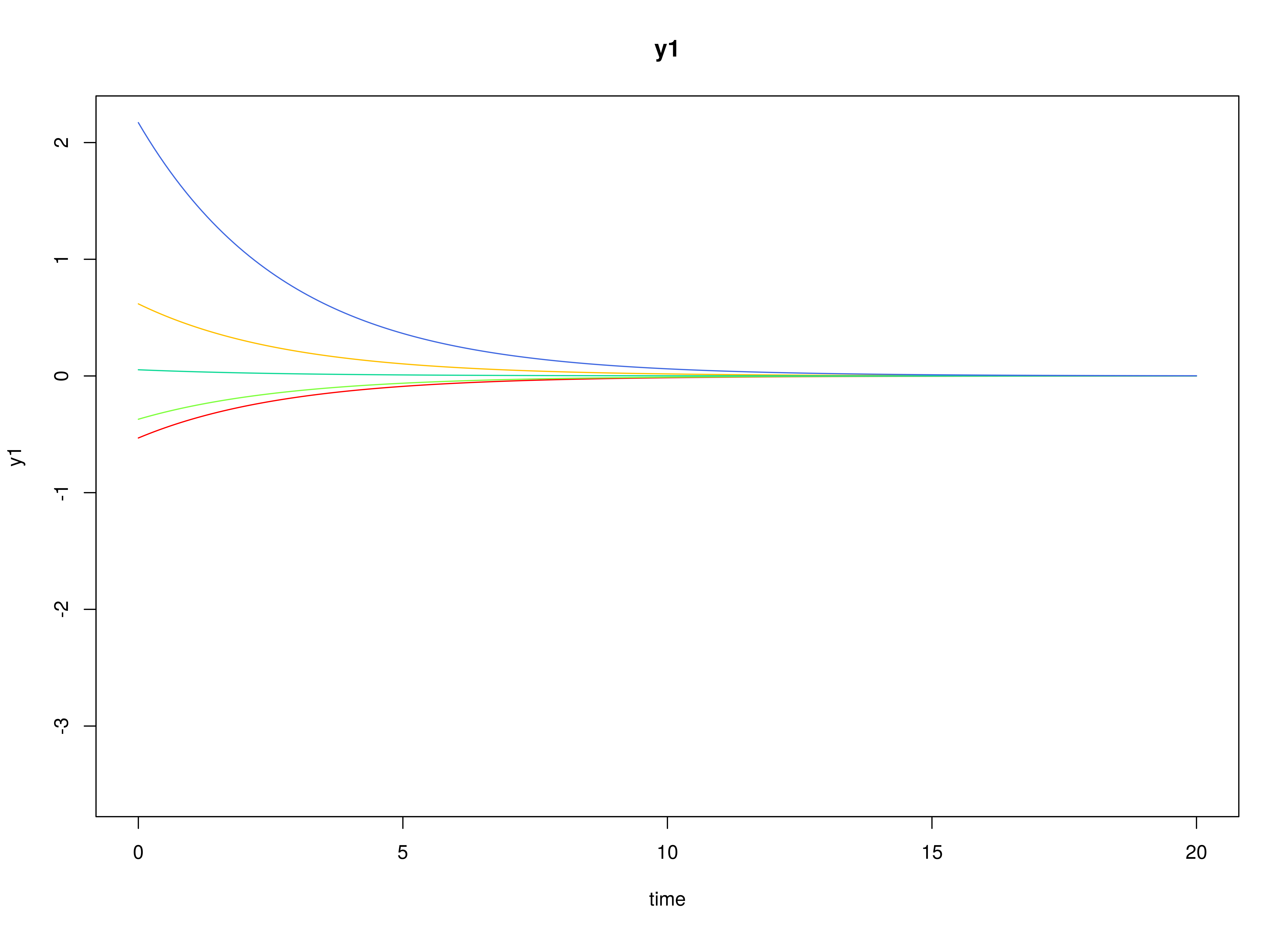
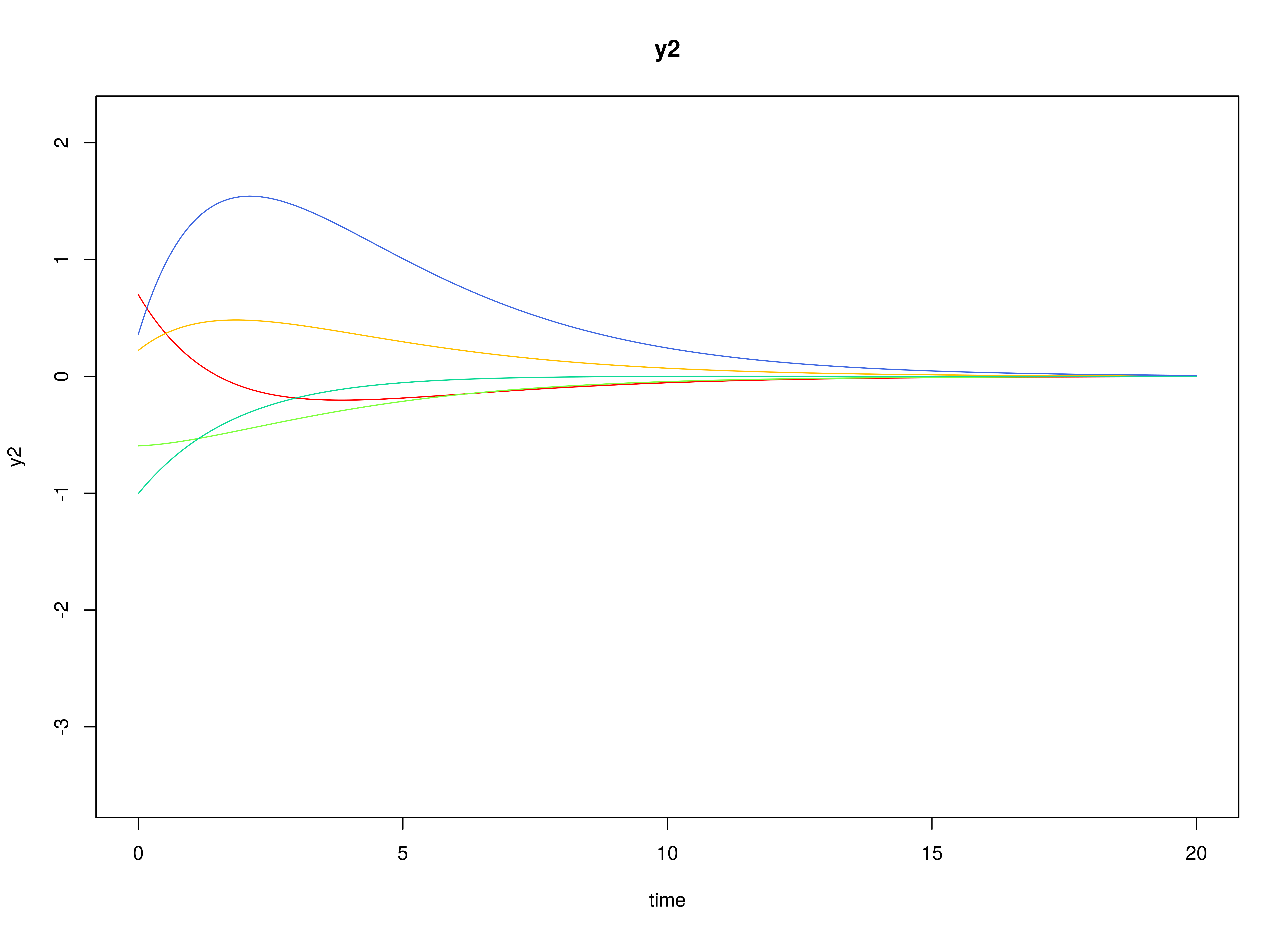
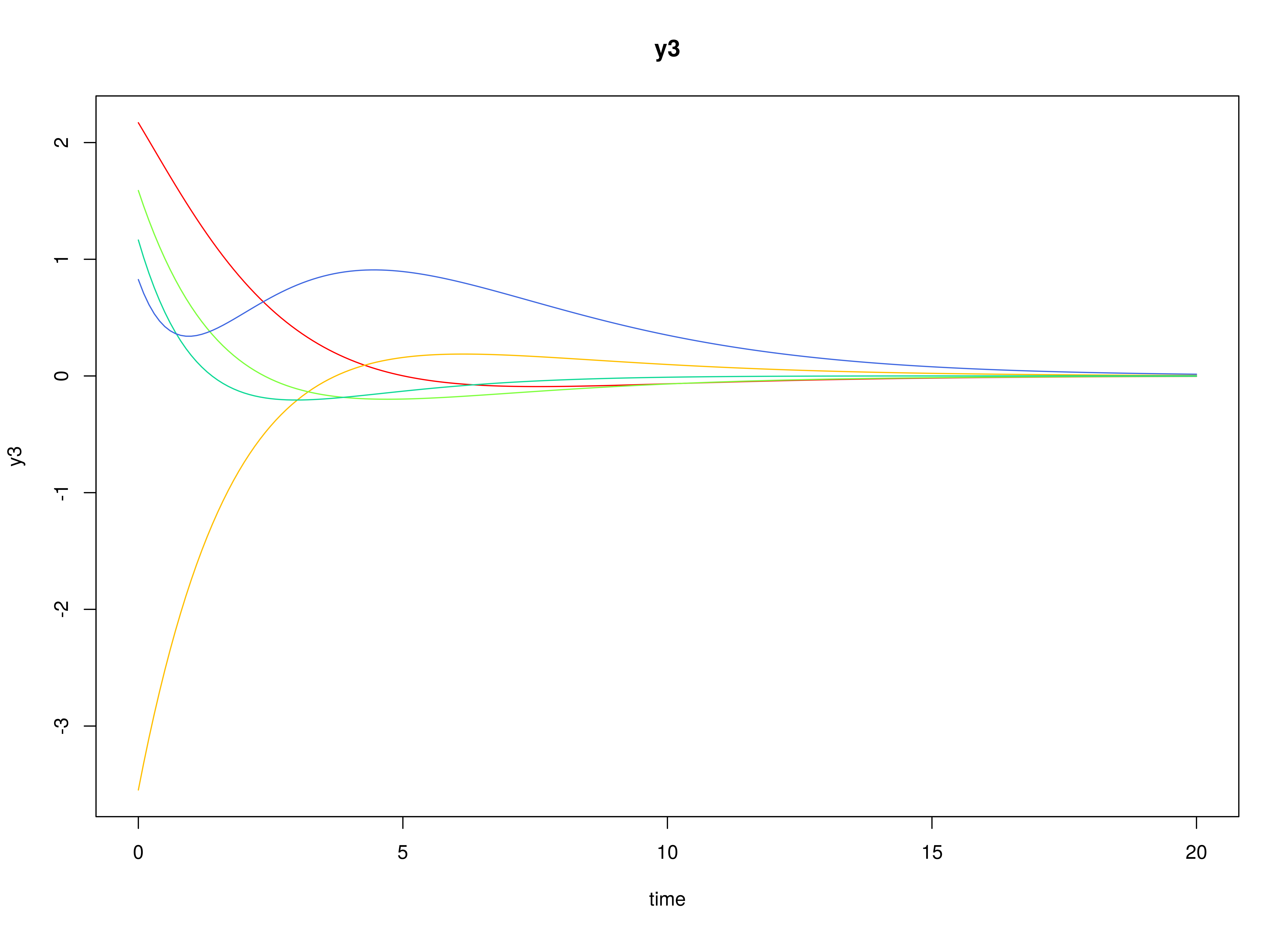
#> [3,]  0.0  0.0  0.2

Visualizing the Dynamics Without Measurement Error and Process Noise (n = 5 with Different Initial Condition)

Using the SimSSMOUFixed Function from the simStateSpace Package to Simulate Data

library(simStateSpace)
sim <- SimSSMOUFixed(
  n = n,
  time = time,
  delta_t = delta_t,
  mu0 = mu0,
  sigma0_l = sigma0_l,
  mu = mu,
  phi = phi,
  sigma_l = sigma_l,
  nu = nu,
  lambda = lambda,
  theta_l = theta_l,
  type = 0
)
data <- as.data.frame(sim)
head(data)
#>   id time          y1          y2        y3
#> 1  1  0.0  0.29937539 -1.37581548 1.3779071
#> 2  1  0.1 -0.98770381 -0.03632195 0.8363080
#> 3  1  0.2  0.33221051 -0.40321664 1.2054318
#> 4  1  0.3 -0.09485392 -0.82030556 1.0272653
#> 5  1  0.4 -1.50322069 -0.36841853 0.1821731
#> 6  1  0.5 -0.75049839  0.35752476 0.2862544
plot(sim)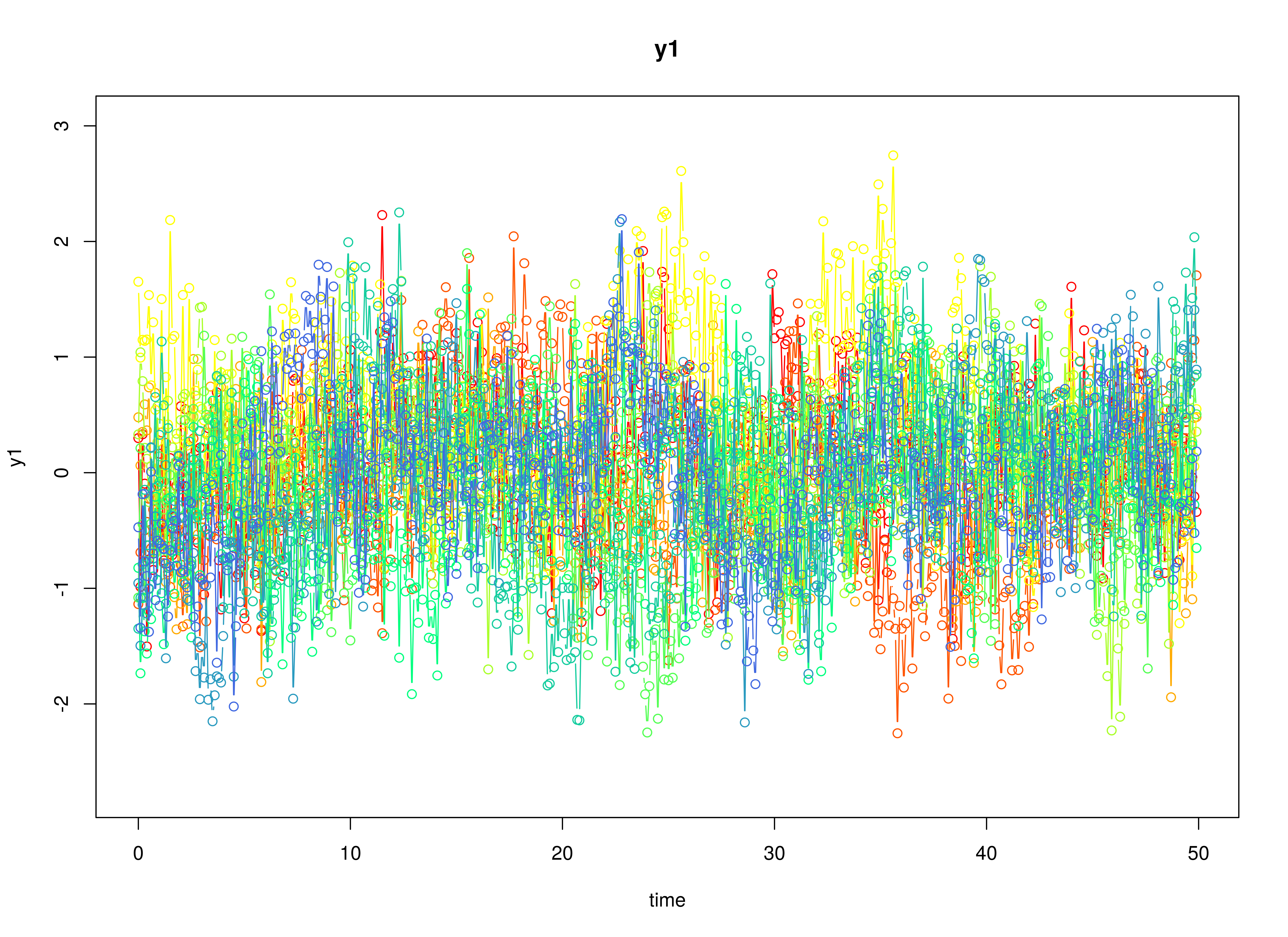

Model Fitting

The FitCTVARIDMx function fits a CT-VAR model on each individual $i$. The argument theta_fixed = FALSE is used here to model the measurement error variances.

library(fitCTVARMx)
fit <- FitCTVARIDMx(
  data = data,
  observed = paste0("y", seq_len(k)),
  id = "id",
  time = "time",
  theta_fixed = FALSE,
  ncores = parallel::detectCores()
)
fit
#> 
#> Means of the estimated paramaters per individual.
#>      phi_11      phi_21      phi_31      phi_12      phi_22      phi_32 
#> -0.99722949  0.95122711 -0.80239749  0.42068315 -0.67971580  1.03223527 
#>      phi_13      phi_23      phi_33    sigma_11    sigma_22    sigma_33 
#> -0.58344255  0.15686252 -0.96351172  0.30496054  0.08162716  0.07656524 
#>    theta_11    theta_22    theta_33 
#>  0.19464192  0.18655239  0.20310336

Multivariate Meta-Analysis

The MetaVARMx function performs multivariate meta-analysis using the estimated parameters and the corresponding sampling variance-covariance matrix for each individual $i$. Estimates with the prefix b0 correspond to the estimates of phi.

library(metaVAR)
meta <- MetaVARMx(
  object = fit,
  random = FALSE,
  ncores = parallel::detectCores()
)
#> Running Model with 9 parameters
#> 
#> Beginning initial fit attempt
#> Running Model with 9 parameters
#> 
#>  Lowest minimum so far:  -64.1091062816891
#> 
#> Solution found

#> 
#>  Solution found!  Final fit=-64.109106 (started at 544.82025)  (1 attempt(s): 1 valid, 0 errors)
#>  Start values from best fit:
#> -0.430268780300005,0.922592460531924,-0.616172503758499,0.0719151003797164,-0.644603539281568,0.80303030596861,-0.110515674133675,0.103613670327686,-0.664549169846479
summary(meta)
#>          est     se        z      p    2.5%   97.5%
#> b0_1 -0.4303 0.1439  -2.9900 0.0028 -0.7123 -0.1482
#> b0_2  0.9226 0.0780  11.8288 0.0000  0.7697  1.0755
#> b0_3 -0.6162 0.0722  -8.5310 0.0000 -0.7577 -0.4746
#> b0_4  0.0719 0.1216   0.5913 0.5543 -0.1665  0.3103
#> b0_5 -0.6446 0.0723  -8.9206 0.0000 -0.7862 -0.5030
#> b0_6  0.8030 0.0667  12.0306 0.0000  0.6722  0.9339
#> b0_7 -0.1105 0.0967  -1.1433 0.2529 -0.3000  0.0789
#> b0_8  0.1036 0.0627   1.6515 0.0986 -0.0194  0.2266
#> b0_9 -0.6645 0.0580 -11.4613 0.0000 -0.7782 -0.5509

References

Cheung, M. W.-L. (2015). Meta‐analysis: A structural equation modeling approach. Wiley. https://doi.org/10.1002/9781118957813

Hunter, M. D. (2017). State space modeling in an open source, modular, structural equation modeling environment. Structural Equation Modeling: A Multidisciplinary Journal, 25(2), 307–324. https://doi.org/10.1080/10705511.2017.1369354

Neale, M. C., Hunter, M. D., Pritikin, J. N., Zahery, M., Brick, T. R., Kirkpatrick, R. M., Estabrook, R., Bates, T. C., Maes, H. H., & Boker, S. M. (2015). OpenMx 2.0: Extended structural equation and statistical modeling. Psychometrika, 81(2), 535–549. https://doi.org/10.1007/s11336-014-9435-8

R Core Team. (2024). R: A language and environment for statistical computing. R Foundation for Statistical Computing. https://www.R-project.org/