Monte Carlo Method using Open-Source Software

Ivan Jacob Agaloos Pesigan

Stage 1: Estimation Stage

The estimation stage can be performed in your statistical package of choice. The parameter estimates and the sampling covariance matrix for the simple mediation model are given below.

Parameter Estimates

mu <- c(
  0.872,
  0.745
)
varnames <- c("alpha", "beta")
names(mu) <- varnames
mu
#> alpha  beta 
#> 0.872 0.745

Sampling Covariance Matrix

Sigma <- matrix(
  data = c(
    1.253778e-02,
    5.244734e-06,
    5.244734e-06,
    1.429014e-02
  ),
  nrow = 2
)
rownames(Sigma) <- colnames(Sigma) <- varnames
Sigma
#>              alpha         beta
#> alpha 1.253778e-02 5.244734e-06
#> beta  5.244734e-06 1.429014e-02

The parameter estimates of interest are \(\hat{\alpha} = 0.872\) and \(\hat{\beta} = 0.745\) and their corresponding sampling covariance matrix.

Stage 2: Simulation Stage

In the simulation stage, \(\hat{\alpha}\) and \(\hat{\beta}\) are used as the mean vector \(\mu\). The covariance matrix \(\Sigma\) consists of the corresponding sampling covariance matrix.

R

Simulation

The MASS package can be used in R to generate the sampling distribution of the indirect effect.

library(MASS)
mustar <- mvrnorm(
  n = 20000,
  mu = mu,
  Sigma = Sigma
)
ab <- mustar[, 1] * mustar[, 2]

Plot

hist(ab)

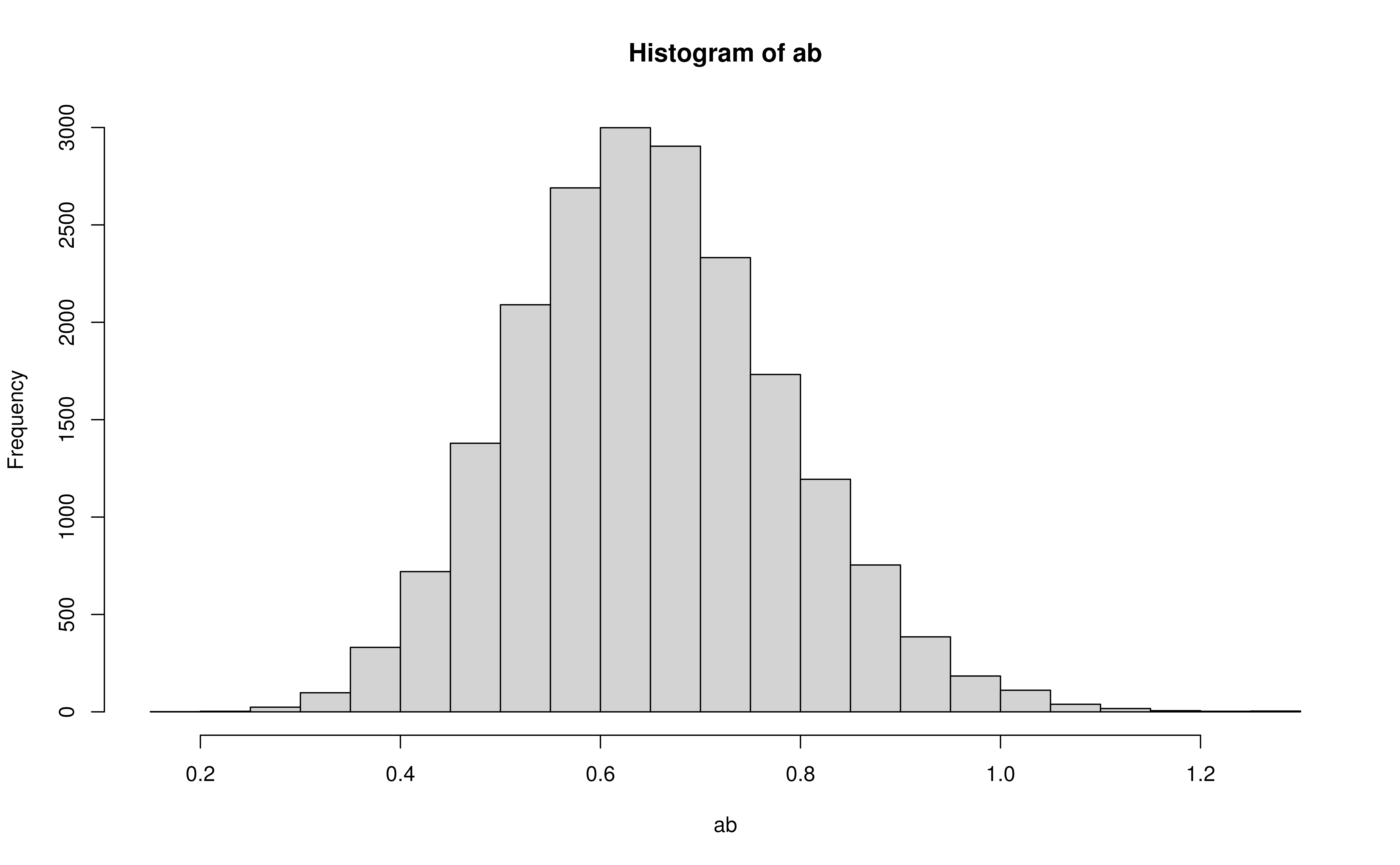
Confidence Intervals

The following corresponds to the \(0.05\), \(0.5\), \(2.5\), \(97.5\), \(99.5\), \(99.95\) percentiles.

quantile(
  x = ab,
  probs = c(0.0005, 0.005, 0.025, 0.975, 0.995, 0.9995)
)
#>     0.05%      0.5%      2.5%     97.5%     99.5%    99.95% 
#> 0.2764884 0.3420248 0.4059116 0.9288212 1.0311513 1.1597367

Python

Simulation

The Numpy module can be used in Python to generate the sampling distribution of the indirect effect.

import numpy as np
mu = [0.872, 0.745]
Sigma = [[1.253778e-02, 5.244734e-06], [5.244734e-06, 1.429014e-02]]
a, b = np.random.default_rng().multivariate_normal(mean = mu, cov = Sigma, size = 20000, method = 'eigh').T
ab = a * b

Confidence Intervals

The following corresponds to the \(0.05\), \(0.5\), \(2.5\), \(97.5\), \(99.5\), \(99.95\) percentiles.

np.percentile(a = ab, q = [0.05, 0.5, 2.5, 97.5, 99.5, 99.95])

array([0.27629, 0.34700399, 0.40509038, 0.92887276, 1.03758102, 1.15662989])

Julia

Simulation

The Distributions.jl package can be used in Julia to generate the sampling distribution of the indirect effect.

using Random, Distributions
mustar = rand(MvNormal([0.872, 0.745], [[1.253778e-02, 5.244734e-06] [5.244734e-06, 1.429014e-02]]), 20000);
a = mustar[1, 1:20000];
b = mustar[2, 1:20000];
ab = a .* b;

Confidence Intervals

The following corresponds to the \(0.05\), \(0.5\), \(2.5\), \(97.5\), \(99.5\), \(99.95\) percentiles.

using StatsBase
percentile(ab, [0.05, 0.5, 2.5, 97.5, 99.5, 99.95])

6-element Vector{Float64}:
 0.2745307698592897
 0.34236235018811184
 0.4054190857337401
 0.9260797738723169
 1.0362695824493815
 1.16103686651973