Benchmark: The Simple Mediation Model with Missing Data using semmcci vs. Nonparametric Bootstrap in lavaan
Ivan Jacob Agaloos Pesigan
2023-09-18
Source:vignettes/benchmark-semmcci.Rmd
benchmark-semmcci.RmdWe compare the Monte Carlo (MC) method with nonparametric bootstrapping (NB) using the simple mediation model with missing data. One advantage of MC over NB is speed. This is because the model is only fitted once in MC whereas it is fitted many times in NB.
Data
n <- 1000
a <- 0.50
b <- 0.50
cp <- 0.25
s2_em <- 1 - a^2
s2_ey <- 1 - cp^2 - a^2 * b^2 - b^2 * s2_em - 2 * cp * a * b
em <- rnorm(n = n, mean = 0, sd = sqrt(s2_em))
ey <- rnorm(n = n, mean = 0, sd = sqrt(s2_ey))
X <- rnorm(n = n)
M <- a * X + em
Y <- cp * X + b * M + ey
df <- data.frame(X, M, Y)

# Create data set with missing values.

miss <- sample(1:dim(df)[1], 300)
df[miss[1:100], "X"] <- NA
df[miss[101:200], "M"] <- NA
df[miss[201:300], "Y"] <- NA
Model Specification
The indirect effect is defined by the product of the slopes of paths
X to M labeled as a and
M to Y labeled as b. In this
example, we are interested in the confidence intervals of
indirect defined as the product of a and
b using the := operator in the
lavaan model syntax.
model <- "
  Y ~ cp * X + b * M
  M ~ a * X
  indirect := a * b
  direct := cp
  total := cp + (a * b)
"
Model Fitting
We can now fit the model using the sem() function from
lavaan. We are using missing = "fiml" to
handle missing data in lavaan. Since there are missing
values in x, we also set fixed.x = FALSE.
fit <- sem(data = df, model = model, missing = "fiml", fixed.x = FALSE)Monte Carlo Confidence Intervals
The fit lavaan object can then be passed to
the MC() function from semmcci to generate
Monte Carlo confidence intervals.
MC(fit, R = 5000L, alpha = c(0.001, 0.01, 0.05))
#> Monte Carlo Confidence Intervals
#>              est     se    R   0.05%    0.5%    2.5%  97.5%  99.5% 99.95%
#> cp        0.2335 0.0292 5000  0.1411  0.1559  0.1756 0.2892 0.3087 0.3262
#> b         0.5112 0.0301 5000  0.4102  0.4314  0.4527 0.5709 0.5861 0.6074
#> a         0.4809 0.0283 5000  0.3900  0.4107  0.4247 0.5368 0.5534 0.5746
#> Y~~Y      0.5542 0.0269 5000  0.4700  0.4874  0.5024 0.6067 0.6221 0.6432
#> M~~M      0.7564 0.0360 5000  0.6400  0.6610  0.6846 0.8249 0.8496 0.8780
#> X~~X      1.0591 0.0487 5000  0.8950  0.9311  0.9647 1.1547 1.1793 1.2202
#> Y~1      -0.0127 0.0250 5000 -0.0938 -0.0753 -0.0615 0.0351 0.0483 0.0673
#> M~1      -0.0223 0.0289 5000 -0.1152 -0.1005 -0.0791 0.0350 0.0485 0.0676
#> X~1       0.0025 0.0332 5000 -0.1009 -0.0818 -0.0621 0.0682 0.0881 0.1025
#> indirect  0.2458 0.0201 5000  0.1845  0.1963  0.2073 0.2871 0.3008 0.3122
#> direct    0.2335 0.0292 5000  0.1411  0.1559  0.1756 0.2892 0.3087 0.3262
#> total     0.4794 0.0282 5000  0.3759  0.4054  0.4230 0.5318 0.5486 0.5724
Nonparametric Bootstrap Confidence Intervals
Nonparametric bootstrap confidence intervals can be generated in
lavaan using the following.
parameterEstimates(
  sem(
    data = df,
    model = model,
    missing = "fiml",
    fixed.x = FALSE,
    se = "bootstrap",
    bootstrap = 5000L
  )
)
#>         lhs op      rhs    label    est    se      z pvalue ci.lower ci.upper
#> 1         Y  ~        X       cp  0.234 0.030  7.745  0.000    0.175    0.292
#> 2         Y  ~        M        b  0.511 0.031 16.515  0.000    0.451    0.572
#> 3         M  ~        X        a  0.481 0.028 16.956  0.000    0.424    0.537
#> 4         Y ~~        Y           0.554 0.027 20.371  0.000    0.500    0.608
#> 5         M ~~        M           0.756 0.037 20.546  0.000    0.684    0.827
#> 6         X ~~        X           1.059 0.051 20.643  0.000    0.959    1.159
#> 7         Y ~1                   -0.013 0.025 -0.508  0.611   -0.062    0.037
#> 8         M ~1                   -0.022 0.030 -0.750  0.453   -0.081    0.037
#> 9         X ~1                    0.002 0.034  0.075  0.941   -0.062    0.068
#> 10 indirect :=      a*b indirect  0.246 0.021 11.974  0.000    0.207    0.287
#> 11   direct :=       cp   direct  0.234 0.030  7.744  0.000    0.175    0.292
#> 12    total := cp+(a*b)    total  0.479 0.029 16.666  0.000    0.422    0.536
Benchmark
Arguments
| Variables | Values | Notes |
|---|---|---|
| R | 5000 | Number of Monte Carlo replications. |
| B | 5000 | Number of bootstrap samples. |
benchmark01 <- microbenchmark(
MC = {
fit <- sem(
data = df,
model = model,
missing = "fiml",
fixed.x = FALSE
)
MC(
fit,
R = R,
decomposition = "chol",
pd = FALSE
)
},
NB = sem(
data = df,
model = model,
missing = "fiml",
fixed.x = FALSE,
se = "bootstrap",
bootstrap = B
),
times = 10
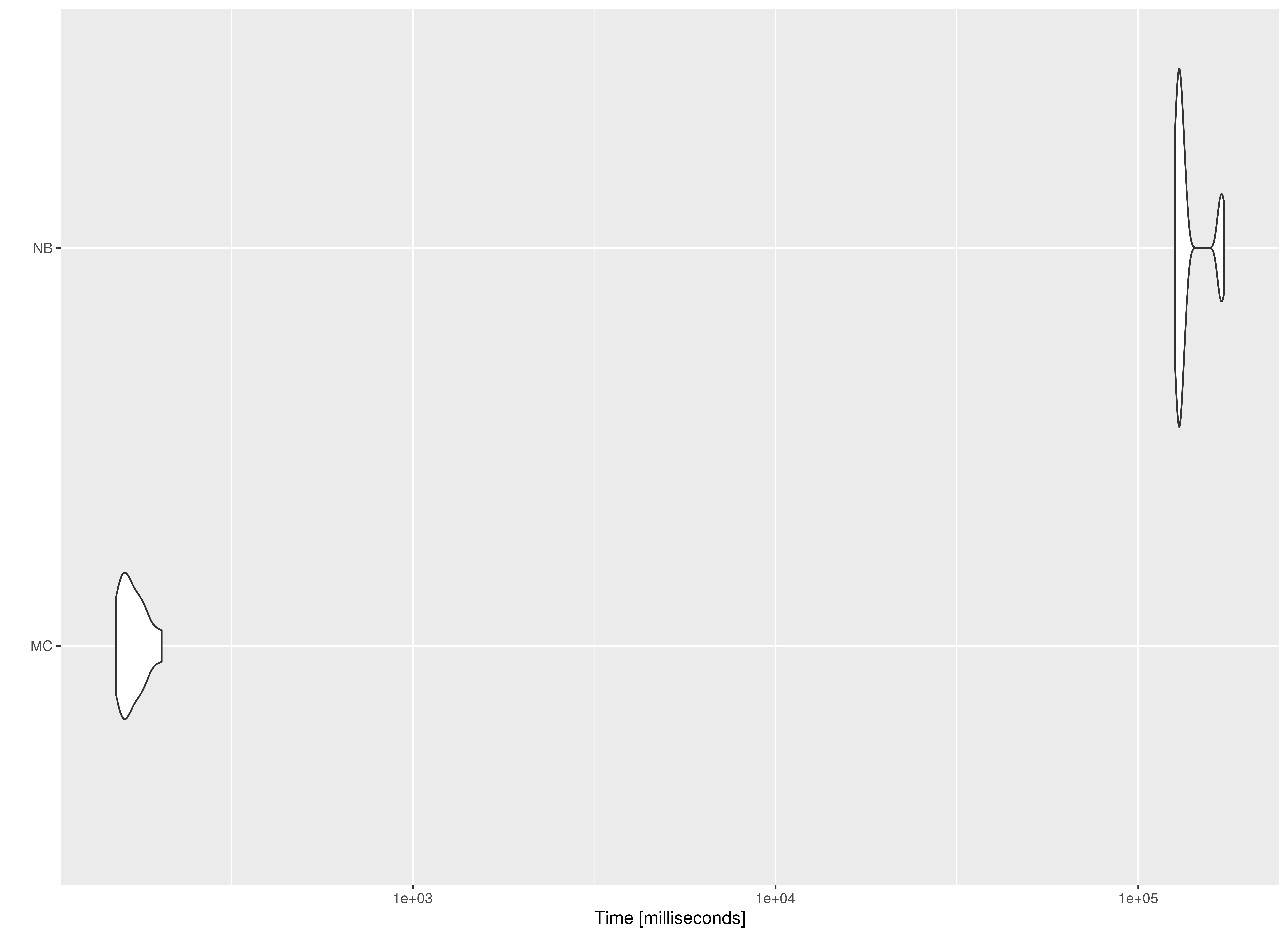
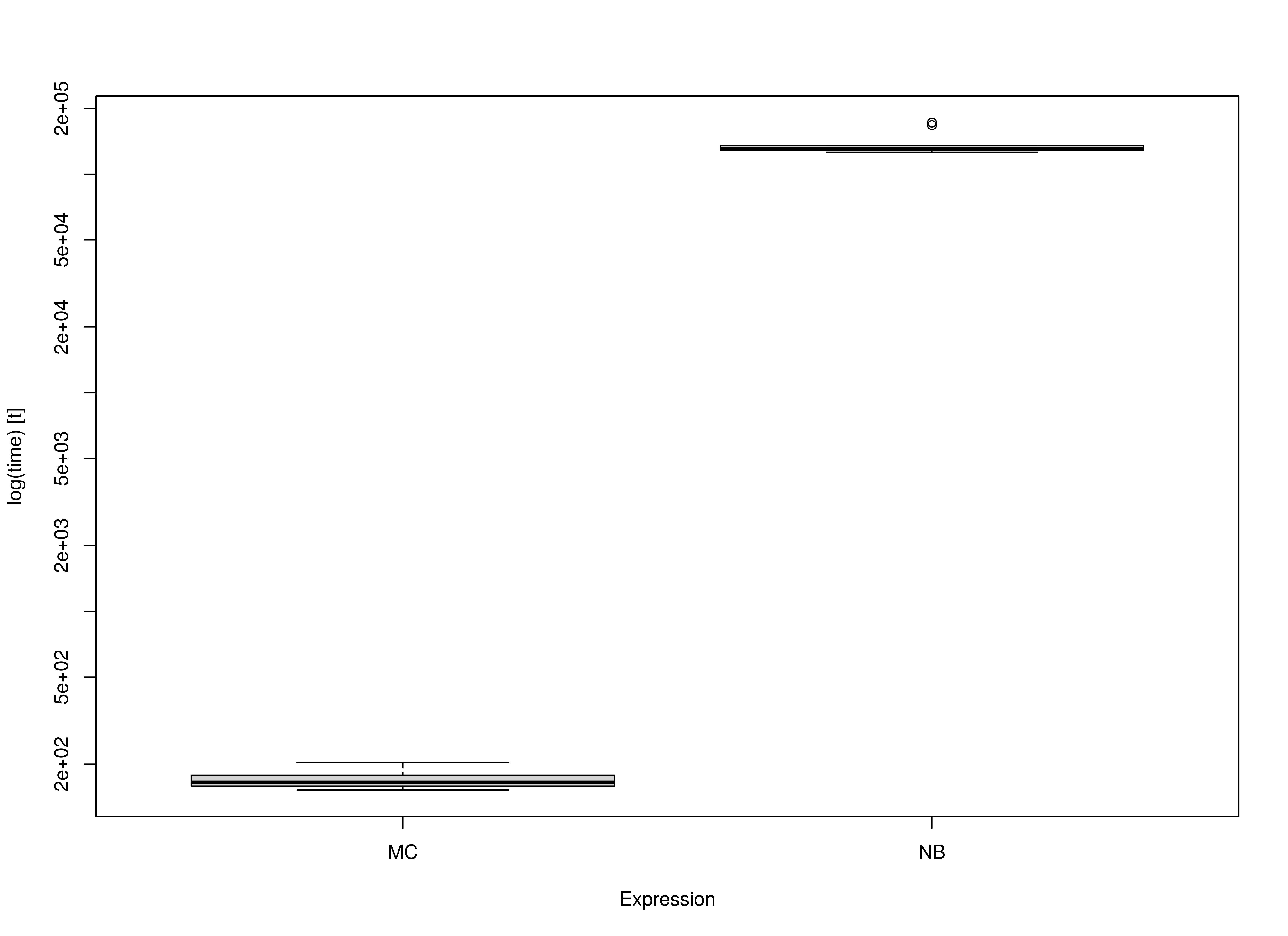
)Summary of Benchmark Results
summary(benchmark01, unit = "ms")
#>   expr         min         lq        mean      median          uq         max
#> 1   MC    264.1755    291.874    310.6323    316.4606    325.2278    361.7557
#> 2   NB 160407.1497 168752.780 173510.1185 174153.1592 178616.3559 187729.1353
#>   neval cld
#> 1    10  a
#> 2    10   b
Summary of Benchmark Results Relative to the Faster Method
summary(benchmark01, unit = "relative")
#>   expr      min     lq     mean   median       uq     max neval cld
#> 1   MC   1.0000   1.00   1.0000   1.0000   1.0000   1.000    10  a
#> 2   NB 607.1991 578.17 558.5708 550.3155 549.2039 518.939    10   b
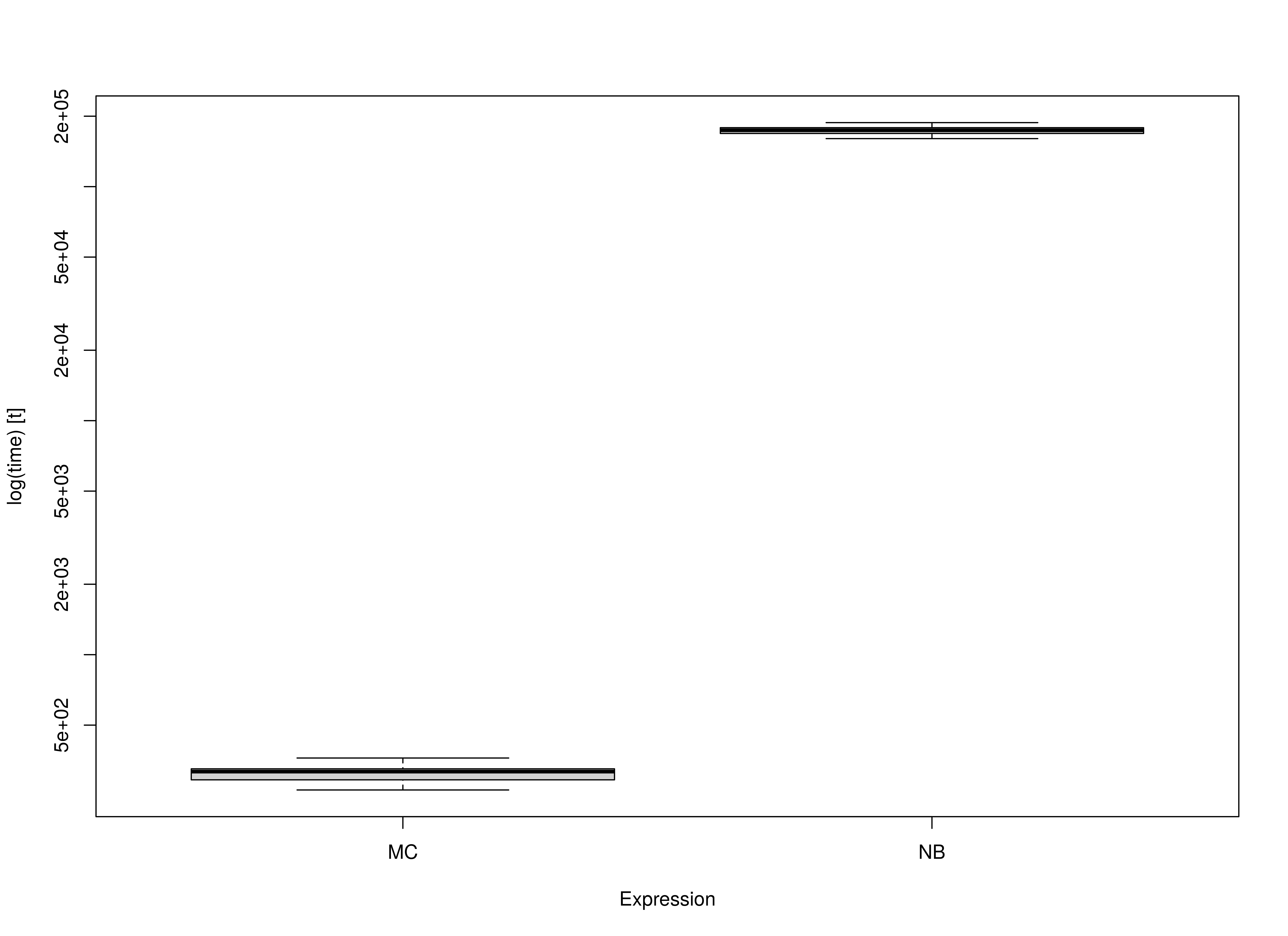
Benchmark - Monte Carlo Method with Precalculated Estimates
fit <- sem(
  data = df,
  model = model,
  missing = "fiml",
  fixed.x = FALSE
)
benchmark02 <- microbenchmark(
  MC = MC(
    fit,
    R = R,
    decomposition = "chol",
    pd = FALSE
  ),
  NB = sem(
    data = df,
    model = model,
    missing = "fiml",
    fixed.x = FALSE,
    se = "bootstrap",
    bootstrap = B
  ),
  times = 10
)
Summary of Benchmark Results
summary(benchmark02, unit = "ms")
#>   expr         min          lq        mean      median          uq         max
#> 1   MC    152.3004    158.5581    169.9283    165.0343    178.1274    203.2036
#> 2   NB 126137.7804 128452.4631 138057.3841 130836.2441 135203.0086 172027.5560
#>   neval cld
#> 1    10  a
#> 2    10   b
Summary of Benchmark Results Relative to the Faster Method
summary(benchmark02, unit = "relative")
#>   expr      min       lq    mean   median       uq      max neval cld
#> 1   MC   1.0000   1.0000   1.000   1.0000   1.0000   1.0000    10  a
#> 2   NB 828.2171 810.1287 812.445 792.7821 759.0241 846.5772    10   b