The Stable Trait, Autoregressive Trait, and State Model

Overview

The stable trait, autoregressive trait, and state (STARTS) model divides a variable measured repeatedly on the same individuals into three parts (Kenny & Zautra, 1995, 2001). Take life satisfaction measured once a year. Part of it is a stable trait that does not change over the study. Part of it is an autoregressive trait that changes slowly: a good year tends to be followed by a fairly good year. The rest is a state that belongs to one occasion only, such as the mood on the day of the survey or measurement error. The model estimates how much of the variance belongs to each part and how strongly the autoregressive part carries over.

The STARTS model is usually fitted as a structural equation model (SEM). It can also be written as a state space model: the stable trait is a latent state that never changes, the autoregressive trait is a latent state with first-order dynamics, and the state part is the measurement error.

This tutorial does three things:

It writes the STARTS model as a state space model.
It simulates data from the model with SimSSMFixed().
It fits the model to the simulated data with dynr (state space) and with lavaan (SEM), and compares both sets of estimates with the values used to simulate the data.

No prior knowledge of state space models is needed.

Model

The measurement model is given by \[\begin{equation} Y_{i, t} = \left( \begin{array}{cc} 1 & 1 \\ \end{array} \right) \left( \begin{array}{c} \eta_{1_{i, t}} \\ \eta_{2_{i, t}} \\ \end{array} \right) + \varepsilon_{i, t}, \quad \mathrm{with} \quad \varepsilon_{i, t} \sim \mathcal{N} \left( 0, \theta \right) \end{equation}\] where \(Y_{i, t}\) is the observed variable at time \(t\) and individual \(i\), \(\eta_{1_{i, t}}\) is the stable trait, \(\eta_{2_{i, t}}\) is the autoregressive trait, and \(\varepsilon_{i, t}\) is the state. \(\theta\) is the variance of the state.

In words, the observed score is the sum of the three parts. The state \(\varepsilon_{i, t}\) is new on every occasion and does not carry over, so it plays the role of measurement error in a state space model.

The dynamic structure is given by \[\begin{equation} \left( \begin{array}{c} \eta_{1_{i, t}} \\ \eta_{2_{i, t}} \\ \end{array} \right) = \left( \begin{array}{cc} 1 & 0 \\ 0 & \beta_{22} \\ \end{array} \right) \left( \begin{array}{c} \eta_{1_{i, t - 1}} \\ \eta_{2_{i, t - 1}} \\ \end{array} \right) + \left( \begin{array}{c} 0 \\ \zeta_{2_{i, t}} \\ \end{array} \right), \quad \mathrm{with} \quad \zeta_{2_{i, t}} \sim \mathcal{N} \left( 0, \psi_{22} \right) . \end{equation}\]

In words, the stable trait stays the same over time. The autoregressive trait keeps a proportion \(\beta_{22}\) of its previous value and adds a new part with variance \(\psi_{22}\). The closer \(\beta_{22}\) is to 1, the more slowly the autoregressive trait changes.

The initial condition is given by \[\begin{equation} \boldsymbol{\eta}_{i, 0} \sim \mathcal{N} \left( \left( \begin{array}{c} \mu_{1} \\ 0 \\ \end{array} \right), \left( \begin{array}{cc} \sigma_{11} & 0 \\ 0 & \sigma_{22} \\ \end{array} \right) \right) . \end{equation}\]

Here, \(\mu_{1}\) is the average stable trait and \(\sigma_{11}\) is how much individuals differ in it. The autoregressive trait has mean zero, because the stable trait carries the mean, and \(\sigma_{22}\) is its variance at the first occasion. The two traits are uncorrelated.

Diagrams

Path diagram of the STARTS model.

The STARTS model as a path diagram, for the first three occasions. The stable trait \(\eta_{1}\) loads on every occasion with a loading of 1. The autoregressive trait \(\eta_{2}\) carries over from one occasion to the next with the autoregressive effect \(\beta_{22}\) and gets a new part \(\zeta_{2}\), with variance \(\psi_{22}\), on each occasion. The state \(\varepsilon\), with variance \(\theta\), is new on every occasion.

State space form of the STARTS model.

The same model in state space form. All the latent variables at one occasion form the state vector \(\boldsymbol{\eta}_{t}\), and all the observed variables form \(\mathbf{y}_{t}\). \(\boldsymbol{\beta}\) carries the state from one occasion to the next, \(\boldsymbol{\Lambda}\) maps the state to the observed variables, \(\boldsymbol{\Psi}\) is the covariance matrix of the process noise \(\boldsymbol{\zeta}_{t}\), and \(\boldsymbol{\Theta}\) is the variance of the state. SimSSMFixed() takes beta, lambda, and the Cholesky factors of \(\boldsymbol{\Psi}\) and \(\boldsymbol{\Theta}\) (psi_l and theta_l).

Data Generation

Notation

Let \(t = 10\) be the number of time points and \(n = 10000\) be the number of individuals. The STARTS model needs many occasions to tell the three parts apart, so this example has more occasions than the other vignettes.

Let the stable trait have mean \(\mu_{1} = 3\) and variance \(\sigma_{11} = 0.5\). Let the autoregressive effect be \(\beta_{22} = 0.6\), the process noise variance \(\psi_{22} = 0.32\), and the state variance \(\theta = 0.3\).

The autoregressive trait starts from its stationary distribution, so its variance at the first occasion is the variance it keeps at every later occasion,

\[\begin{equation} \sigma_{22} = \frac{\psi_{22}}{1 - \beta_{22}^{2}} = 0.5 . \end{equation}\]

With these values, the stable trait, the autoregressive trait, and the state contribute 0.5, 0.5, and 0.3 to the variance of the observed score on every occasion.

R Function Arguments

The simulation functions take covariance matrices as lower triangular Cholesky factors (the arguments ending in _l). Because the stable trait has no process noise, psi has a row and a column of zeros, and its Cholesky factor is written directly.

n
#> [1] 10000
time
#> [1] 10
mu0
#> [1] 3 0
sigma0
#>      [,1] [,2]
#> [1,]  0.5  0.0
#> [2,]  0.0  0.5
sigma0_l # sigma0_l <- t(chol(sigma0))
#>           [,1]      [,2]
#> [1,] 0.7071068 0.0000000
#> [2,] 0.0000000 0.7071068
alpha
#> [1] 0 0
beta
#>      [,1] [,2]
#> [1,]    1  0.0
#> [2,]    0  0.6
psi
#>      [,1] [,2]
#> [1,]    0 0.00
#> [2,]    0 0.32
psi_l
#>      [,1]      [,2]
#> [1,]    0 0.0000000
#> [2,]    0 0.5656854
nu
#> [1] 0
lambda
#>      [,1] [,2]
#> [1,]    1    1
theta
#>      [,1]
#> [1,]  0.3
theta_l # theta_l <- t(chol(theta))
#>           [,1]
#> [1,] 0.5477226

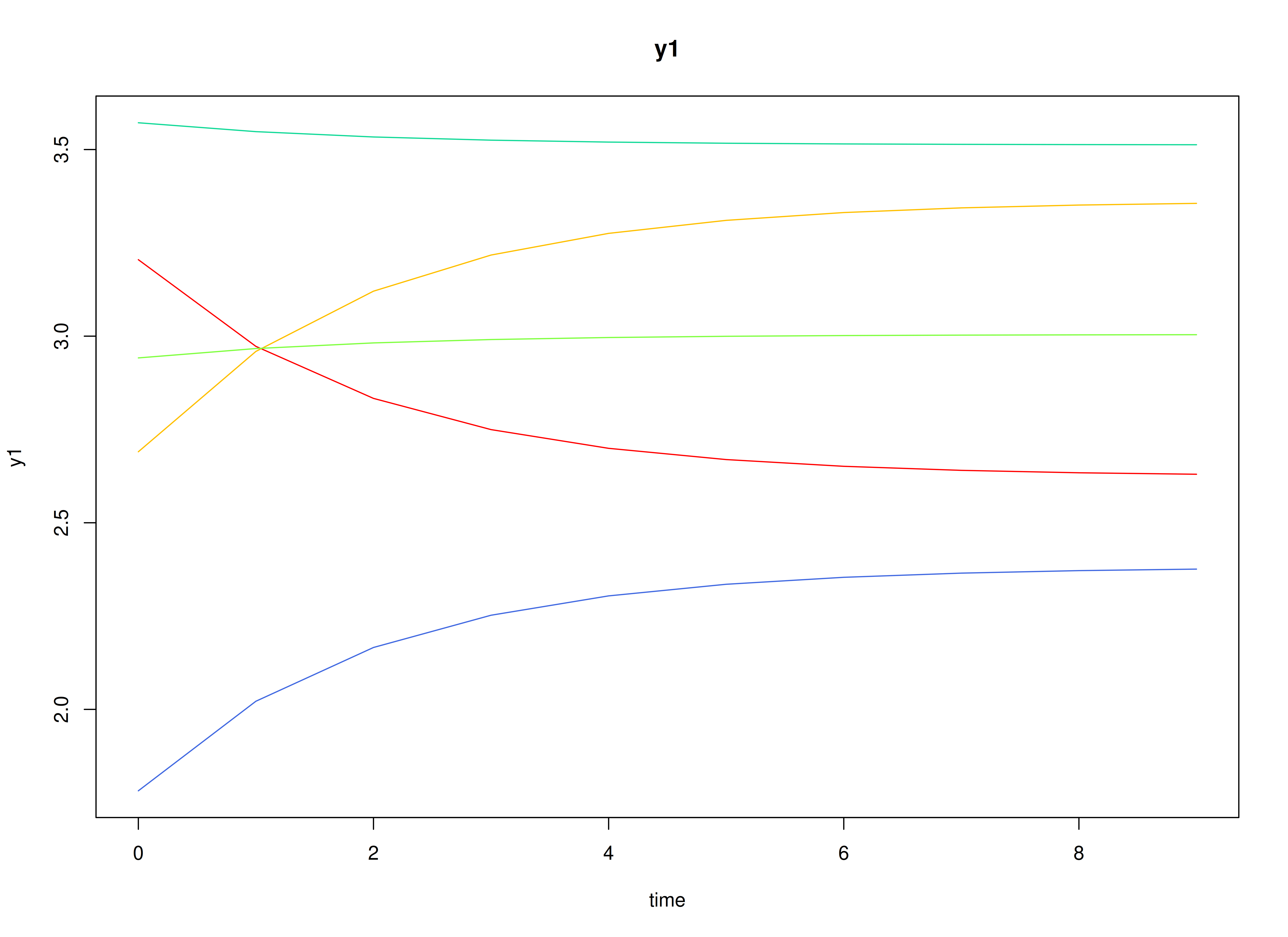
Visualizing the Dynamics Without Process Noise and Measurement Error (n = 5 with Different Initial Condition)

Without process noise and the state, each individual’s autoregressive trait decays toward zero, so each trajectory settles at the individual’s stable trait.

Using the `SimSSMFixed` Function from the `simStateSpace` Package to Simulate Data

Now we add the process noise and the state and simulate the full data set. as.data.frame() returns the data in long format, one row per individual and time point, with the columns id, time, and y1.

library(simStateSpace)
sim <- SimSSMFixed(
  n = n,
  time = time,
  mu0 = mu0,
  sigma0_l = sigma0_l,
  alpha = alpha,
  beta = beta,
  psi_l = psi_l,
  nu = nu,
  lambda = lambda,
  theta_l = theta_l,
  type = 0
)
data <- as.data.frame(sim)
head(data)
#>   id time       y1
#> 1  1    0 2.724102
#> 2  1    1 2.554146
#> 3  1    2 2.834498
#> 4  1    3 1.952812
#> 5  1    4 1.715812
#> 6  1    5 1.798422
summary(data)
#>        id             time           y1        
#>  Min.   :    1   Min.   :0.0   Min.   :-1.844  
#>  1st Qu.: 2501   1st Qu.:2.0   1st Qu.: 2.230  
#>  Median : 5000   Median :4.5   Median : 3.006  
#>  Mean   : 5000   Mean   :4.5   Mean   : 3.007  
#>  3rd Qu.: 7500   3rd Qu.:7.0   3rd Qu.: 3.778  
#>  Max.   :10000   Max.   :9.0   Max.   : 8.039
plot(sim)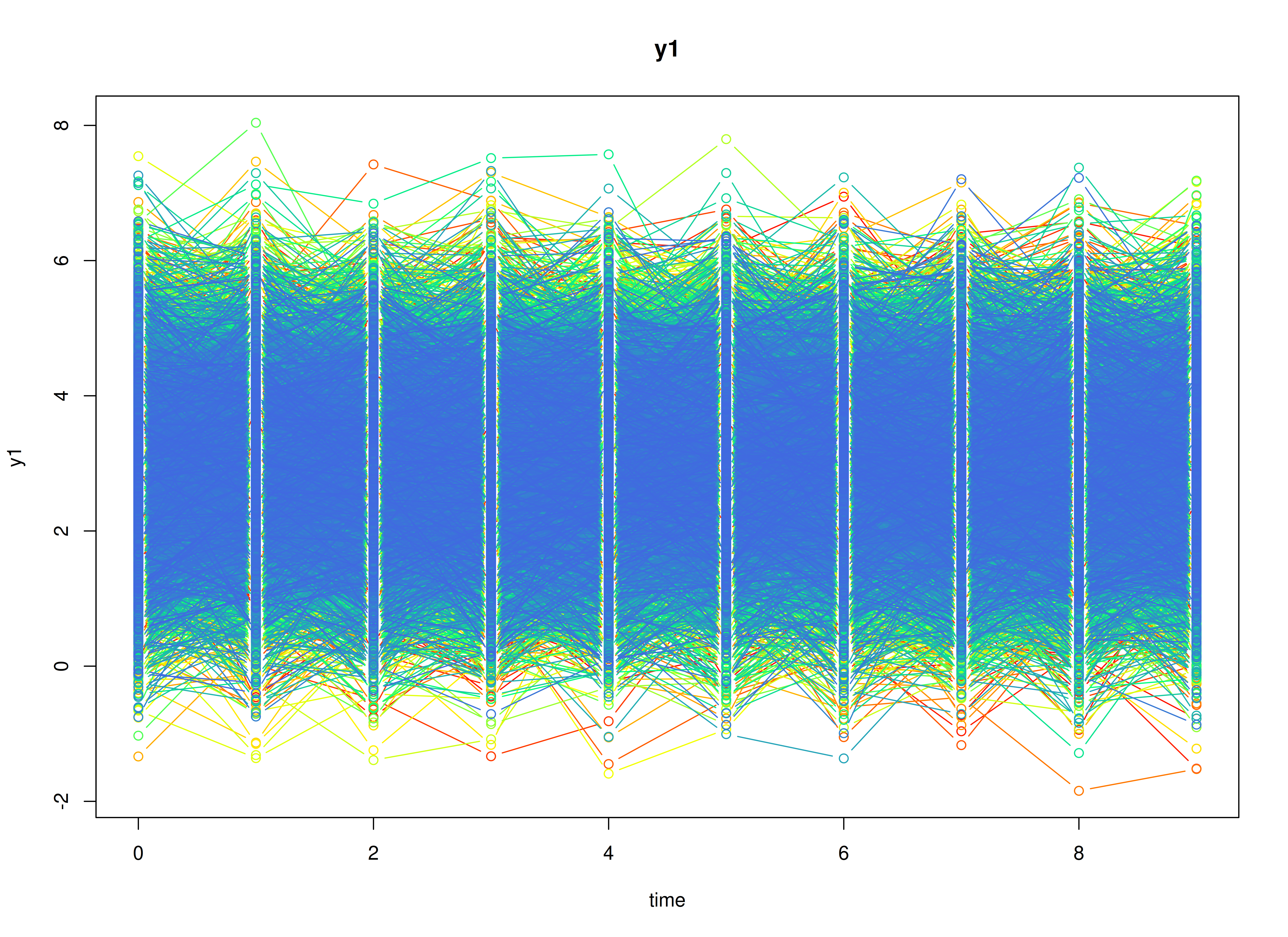

Model Fitting

We first fit the model with dynr, which estimates state space models by maximum likelihood using the Kalman filter.

A dynr model is built from pieces that match the equations above: the data, the initial condition, the measurement model, the dynamic model, and the noise. Each parameter gets a name (for example, beta_2_2 for \(\beta_{22}\)), and the same name used in two places means one shared parameter. The starting values are set to the population values for convenience; with real data, they would be rough guesses.

Prepare Data

Tell dynr which columns hold the individual, the time, and the observed variables.

dynr_data <- dynr::dynr.data(
  dataframe = data,
  id = "id",
  time = "time",
  observed = "y1"
)

Prepare Initial Condition

The mean of the stable trait and the variances of both traits at the first occasion are estimated. The mean of the autoregressive trait and the covariance of the two traits are fixed at zero.

dynr_initial <- dynr::prep.initial(
  values.inistate = mu0,
  params.inistate = c("mu0_1_1", "fixed"),
  values.inicov = sigma0,
  params.inicov = matrix(
    data = c(
      "sigma0_1_1", "fixed",
      "fixed", "sigma0_2_2"
    ),
    nrow = 2
  )
)

Prepare Measurement Model

The loadings \(\left( 1, 1 \right)\) are fixed.

dynr_measurement <- dynr::prep.measurement(
  values.load = lambda,
  params.load = matrix(data = "fixed", nrow = 1, ncol = 2),
  state.names = c("eta_1", "eta_2"),
  obs.names = "y1"
)

Prepare Dynamic Process

The stable trait carries over unchanged; the autoregressive trait has the autoregressive effect \(\beta_{22}\).

dynr_dynamics <- dynr::prep.formulaDynamics(
  formula = list(
    eta_1 ~ eta_1,
    eta_2 ~ beta_2_2 * eta_2
  ),
  startval = c(beta_2_2 = beta[2, 2]),
  isContinuousTime = FALSE
)

Prepare Process Noise

Only the autoregressive trait has process noise. The state variance \(\theta\) is estimated.

dynr_noise <- dynr::prep.noise(
  values.latent = psi,
  params.latent = matrix(
    data = c(
      "fixed", "fixed",
      "fixed", "psi_2_2"
    ),
    nrow = 2
  ),
  values.observed = theta,
  params.observed = "theta"
)

Prepare the Model

The pieces are put together into one model. dynr writes the model as C code to outfile and compiles it.

model <- dynr::dynr.model(
  data = dynr_data,
  initial = dynr_initial,
  measurement = dynr_measurement,
  dynamics = dynr_dynamics,
  noise = dynr_noise,
  outfile = "starts.c"
)

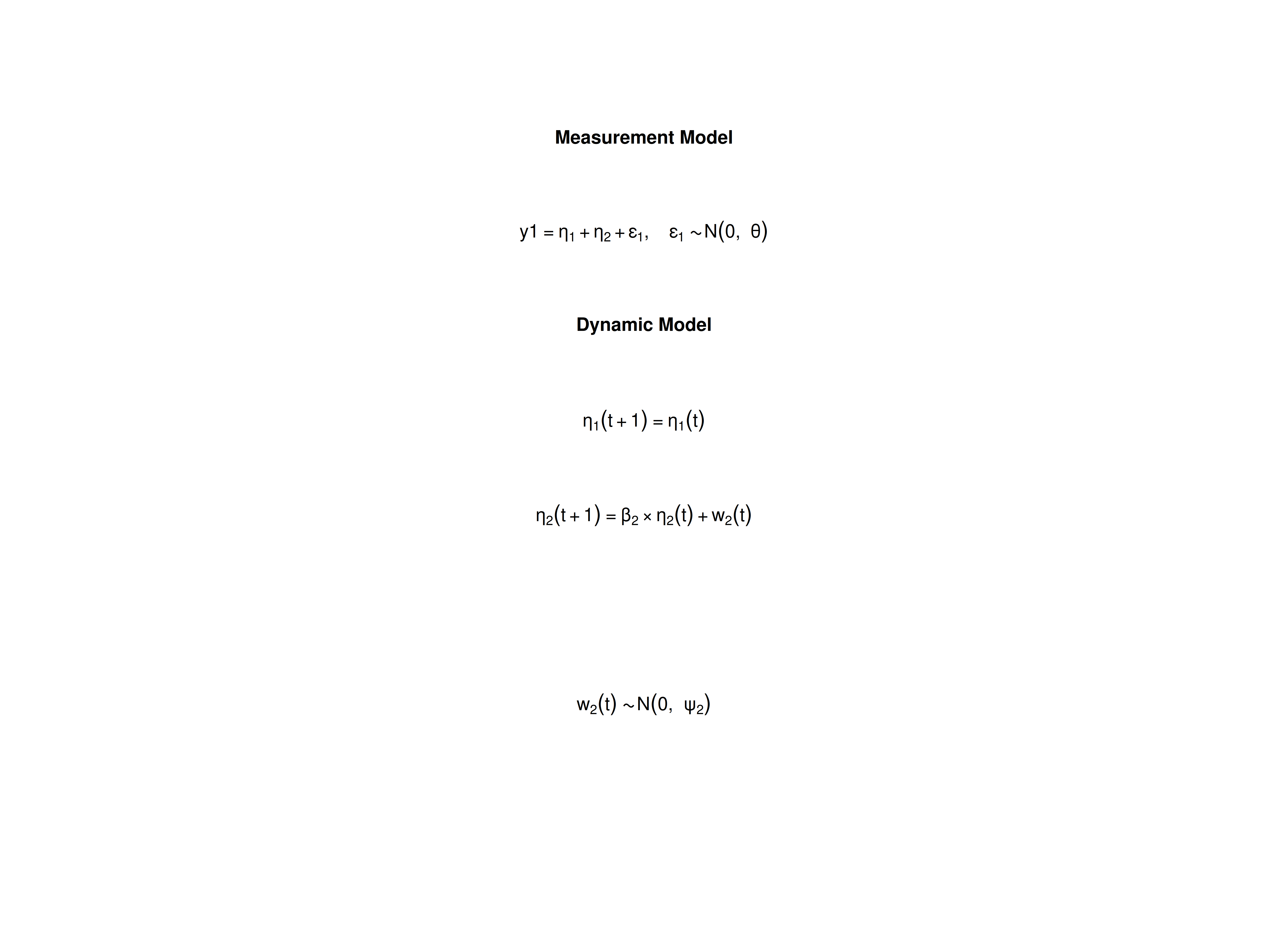
The plot below shows the model equations with the parameter names.

Fit the Model

results <- dynr::dynr.cook(
  model,
  debug_flag = TRUE,
  verbose = FALSE
)
#> [1] "Get ready!!!!"
#> using C compiler: ‘gcc (Ubuntu 15.2.0-16ubuntu1) 15.2.0’
#> Optimization function called.
#> Starting Hessian calculation ...
#> Finished Hessian calculation.
#> Original exit flag:  3 
#> Modified exit flag:  3 
#> Optimization terminated successfully: ftol_rel or ftol_abs was reached. 
#> Original fitted parameters:  0.6069395 -1.138077 -1.195125 3.006529 -0.7009229 
#> -0.7188562 
#> 
#> Transformed fitted parameters:  0.6069395 0.3204346 0.3026661 3.006529 
#> 0.4961272 0.4873093 
#> 
#> Doing end processing
#> Successful trial
#> Total Time: 46.7627 
#> Backend Time: 46.39977

Summary

The summary lists each estimate with its standard error, \(t\) value, confidence interval, and \(p\) value.

summary(results)
#> Coefficients:
#>            Estimate Std. Error t value ci.lower ci.upper            Pr(>|t|)
#> beta_2_2   0.606940   0.012620   48.09 0.582205 0.631674 <0.0000000000000002
#> psi_2_2    0.320435   0.009594   33.40 0.301631 0.339238 <0.0000000000000002
#> theta      0.302666   0.008010   37.79 0.286967 0.318366 <0.0000000000000002
#> mu0_1_1    3.006529   0.008286  362.83 2.990288 3.022770 <0.0000000000000002
#> sigma0_1_1 0.496127   0.010921   45.43 0.474722 0.517532 <0.0000000000000002
#> sigma0_2_2 0.487309   0.015438   31.57 0.457051 0.517567 <0.0000000000000002
#>               
#> beta_2_2   ***
#> psi_2_2    ***
#> theta      ***
#> mu0_1_1    ***
#> sigma0_1_1 ***
#> sigma0_2_2 ***
#> ---
#> Signif. codes:  0 '***' 0.001 '**' 0.01 '*' 0.05 '.' 0.1 ' ' 1
#> 
#> -2 log-likelihood value at convergence = 260347.42
#> AIC = 260359.42
#> BIC = 260416.49

The STARTS Model in Structural Equation Modeling

The same model in SEM form, fitted with lavaan, should give nearly the same estimates. In SEM, each occasion is a separate observed variable in one row per individual (wide format). The stable trait is a factor with loadings of 1 on all occasions, and the autoregressive trait is a factor on each occasion with a loading of 1 on that occasion.

Wide Data Set

as.data.frame() with long = FALSE returns the data in wide format.

data <- as.data.frame(sim, long = FALSE)
head(data)
#>   id     y1_0      y1_1     y1_2     y1_3     y1_4         y1_5      y1_6
#> 1  1 2.724102 2.5541457 2.834498 1.952812 1.715812  1.798422003 2.6524161
#> 2  2 1.398728 1.5898005 2.078358 3.136913 3.420155  1.656597551 1.7696126
#> 3  3 5.130244 3.5302297 3.728487 3.017891 5.113005  4.727711315 3.2796103
#> 4  4 1.891987 1.9632526 3.094126 1.995233 2.613028  2.185718347 3.3743940
#> 5  5 1.725919 0.5120299 0.753101 2.145500 2.795792  2.154440779 1.9059497
#> 6  6 2.957243 1.4160208 1.596537 1.762764 1.159233 -0.005812339 0.8095458
#>        y1_7      y1_8      y1_9
#> 1 2.0029863 2.4650079 2.7663724
#> 2 0.6304025 1.7566680 0.4364570
#> 3 2.7692017 3.2305090 3.4921984
#> 4 2.7263657 0.8028354 1.1643963
#> 5 1.7443716 1.6288711 0.7896516
#> 6 1.5117643 1.3294805 2.4095639

Model

The model has the same structure for every occasion, so we write it with paste0(). The parameter labels match the dynr names. Giving the autoregressive effect, the process noise variance, and the state variance the same label on every occasion constrains them to be equal over time, as in the state space model.

waves <- 0:(time - 1)
now <- waves[-1]
before <- waves[-time]
model <- paste(
  c(
    "# stable trait: loadings fixed at 1",
    paste0("eta_1 =~ ", paste0("1 * y1_", waves, collapse = " + ")),
    "# autoregressive trait on each occasion",
    paste0("ar_", waves, " =~ 1 * y1_", waves),
    "# autoregressive effect",
    paste0("ar_", now, " ~ beta_2_2 * ar_", before),
    "# autoregressive trait at the first occasion",
    "ar_0 ~~ sigma0_2_2 * ar_0",
    "# process noise at later occasions",
    paste0("ar_", now, " ~~ psi_2_2 * ar_", now),
    "# stable trait: mean and variance",
    "eta_1 ~ mu0_1_1 * 1",
    "eta_1 ~~ sigma0_1_1 * eta_1",
    "# the two traits are uncorrelated",
    "eta_1 ~~ 0 * ar_0",
    "# state variance, equal over time; no observed intercepts",
    paste0("y1_", waves, " ~~ theta * y1_", waves),
    paste0("y1_", waves, " ~ 0 * 1")
  ),
  collapse = "\n"
)
cat(model)
#> # stable trait: loadings fixed at 1
#> eta_1 =~ 1 * y1_0 + 1 * y1_1 + 1 * y1_2 + 1 * y1_3 + 1 * y1_4 + 1 * y1_5 + 1 * y1_6 + 1 * y1_7 + 1 * y1_8 + 1 * y1_9
#> # autoregressive trait on each occasion
#> ar_0 =~ 1 * y1_0
#> ar_1 =~ 1 * y1_1
#> ar_2 =~ 1 * y1_2
#> ar_3 =~ 1 * y1_3
#> ar_4 =~ 1 * y1_4
#> ar_5 =~ 1 * y1_5
#> ar_6 =~ 1 * y1_6
#> ar_7 =~ 1 * y1_7
#> ar_8 =~ 1 * y1_8
#> ar_9 =~ 1 * y1_9
#> # autoregressive effect
#> ar_1 ~ beta_2_2 * ar_0
#> ar_2 ~ beta_2_2 * ar_1
#> ar_3 ~ beta_2_2 * ar_2
#> ar_4 ~ beta_2_2 * ar_3
#> ar_5 ~ beta_2_2 * ar_4
#> ar_6 ~ beta_2_2 * ar_5
#> ar_7 ~ beta_2_2 * ar_6
#> ar_8 ~ beta_2_2 * ar_7
#> ar_9 ~ beta_2_2 * ar_8
#> # autoregressive trait at the first occasion
#> ar_0 ~~ sigma0_2_2 * ar_0
#> # process noise at later occasions
#> ar_1 ~~ psi_2_2 * ar_1
#> ar_2 ~~ psi_2_2 * ar_2
#> ar_3 ~~ psi_2_2 * ar_3
#> ar_4 ~~ psi_2_2 * ar_4
#> ar_5 ~~ psi_2_2 * ar_5
#> ar_6 ~~ psi_2_2 * ar_6
#> ar_7 ~~ psi_2_2 * ar_7
#> ar_8 ~~ psi_2_2 * ar_8
#> ar_9 ~~ psi_2_2 * ar_9
#> # stable trait: mean and variance
#> eta_1 ~ mu0_1_1 * 1
#> eta_1 ~~ sigma0_1_1 * eta_1
#> # the two traits are uncorrelated
#> eta_1 ~~ 0 * ar_0
#> # state variance, equal over time; no observed intercepts
#> y1_0 ~~ theta * y1_0
#> y1_1 ~~ theta * y1_1
#> y1_2 ~~ theta * y1_2
#> y1_3 ~~ theta * y1_3
#> y1_4 ~~ theta * y1_4
#> y1_5 ~~ theta * y1_5
#> y1_6 ~~ theta * y1_6
#> y1_7 ~~ theta * y1_7
#> y1_8 ~~ theta * y1_8
#> y1_9 ~~ theta * y1_9
#> y1_0 ~ 0 * 1
#> y1_1 ~ 0 * 1
#> y1_2 ~ 0 * 1
#> y1_3 ~ 0 * 1
#> y1_4 ~ 0 * 1
#> y1_5 ~ 0 * 1
#> y1_6 ~ 0 * 1
#> y1_7 ~ 0 * 1
#> y1_8 ~ 0 * 1
#> y1_9 ~ 0 * 1

lavaan::lavaan() adds nothing to the model by itself, so every parameter above is exactly the one written.

fit <- lavaan::lavaan(
  model = model,
  data = data
)
lavaan::summary(fit)
#> lavaan 0.7-3 ended normally after 35 iterations
#> 
#>   Estimator                                         ML
#>   Optimization method                           NLMINB
#>   Number of model parameters                        31
#>   Number of equality constraints                    25
#> 
#>   Number of observations                         10000
#> 
#> Model Test User Model:
#>                                                       
#>   Test statistic                                51.382
#>   Degrees of freedom                                59
#>   P-value (Chi-square)                           0.749
#>                                                       
#>   Browne's residual (NT model-based) test             
#>   Test statistic                                51.471
#>   Degrees of freedom                                59
#>   P-value (Chi-square)                           0.746
#> 
#> Parameter Estimates:
#> 
#>   Standard errors                             Standard
#>   Information                                 Expected
#>   Information saturated (h1) model          Structured
#> 
#> Latent Variables:
#>                    Estimate  Std.Err  z-value  P(>|z|)
#>   eta_1 =~                                            
#>     y1_0              1.000                           
#>     y1_1              1.000                           
#>     y1_2              1.000                           
#>     y1_3              1.000                           
#>     y1_4              1.000                           
#>     y1_5              1.000                           
#>     y1_6              1.000                           
#>     y1_7              1.000                           
#>     y1_8              1.000                           
#>     y1_9              1.000                           
#>   ar_0 =~                                             
#>     y1_0              1.000                           
#>   ar_1 =~                                             
#>     y1_1              1.000                           
#>   ar_2 =~                                             
#>     y1_2              1.000                           
#>   ar_3 =~                                             
#>     y1_3              1.000                           
#>   ar_4 =~                                             
#>     y1_4              1.000                           
#>   ar_5 =~                                             
#>     y1_5              1.000                           
#>   ar_6 =~                                             
#>     y1_6              1.000                           
#>   ar_7 =~                                             
#>     y1_7              1.000                           
#>   ar_8 =~                                             
#>     y1_8              1.000                           
#>   ar_9 =~                                             
#>     y1_9              1.000                           
#> 
#> Regressions:
#>                    Estimate  Std.Err  z-value  P(>|z|)
#>   ar_1 ~                                              
#>     ar_0    (b_2_)    0.607    0.013   48.421    0.000
#>   ar_2 ~                                              
#>     ar_1    (b_2_)    0.607    0.013   48.421    0.000
#>   ar_3 ~                                              
#>     ar_2    (b_2_)    0.607    0.013   48.421    0.000
#>   ar_4 ~                                              
#>     ar_3    (b_2_)    0.607    0.013   48.421    0.000
#>   ar_5 ~                                              
#>     ar_4    (b_2_)    0.607    0.013   48.421    0.000
#>   ar_6 ~                                              
#>     ar_5    (b_2_)    0.607    0.013   48.421    0.000
#>   ar_7 ~                                              
#>     ar_6    (b_2_)    0.607    0.013   48.421    0.000
#>   ar_8 ~                                              
#>     ar_7    (b_2_)    0.607    0.013   48.421    0.000
#>   ar_9 ~                                              
#>     ar_8    (b_2_)    0.607    0.013   48.421    0.000
#> 
#> Covariances:
#>                    Estimate  Std.Err  z-value  P(>|z|)
#>   eta_1 ~~                                            
#>     ar_0              0.000                           
#> 
#> Intercepts:
#>                    Estimate  Std.Err  z-value  P(>|z|)
#>     eta_1   (m0_1)    3.007    0.008  362.790    0.000
#>    .y1_0              0.000                           
#>    .y1_1              0.000                           
#>    .y1_2              0.000                           
#>    .y1_3              0.000                           
#>    .y1_4              0.000                           
#>    .y1_5              0.000                           
#>    .y1_6              0.000                           
#>    .y1_7              0.000                           
#>    .y1_8              0.000                           
#>    .y1_9              0.000                           
#> 
#> Variances:
#>                    Estimate  Std.Err  z-value  P(>|z|)
#>     ar_0    (s0_2)    0.487    0.015   31.858    0.000
#>    .ar_1    (p_2_)    0.320    0.010   33.268    0.000
#>    .ar_2    (p_2_)    0.320    0.010   33.268    0.000
#>    .ar_3    (p_2_)    0.320    0.010   33.268    0.000
#>    .ar_4    (p_2_)    0.320    0.010   33.268    0.000
#>    .ar_5    (p_2_)    0.320    0.010   33.268    0.000
#>    .ar_6    (p_2_)    0.320    0.010   33.268    0.000
#>    .ar_7    (p_2_)    0.320    0.010   33.268    0.000
#>    .ar_8    (p_2_)    0.320    0.010   33.268    0.000
#>    .ar_9    (p_2_)    0.320    0.010   33.268    0.000
#>     eta_1   (s0_1)    0.496    0.011   45.215    0.000
#>    .y1_0    (thet)    0.303    0.008   37.787    0.000
#>    .y1_1    (thet)    0.303    0.008   37.787    0.000
#>    .y1_2    (thet)    0.303    0.008   37.787    0.000
#>    .y1_3    (thet)    0.303    0.008   37.787    0.000
#>    .y1_4    (thet)    0.303    0.008   37.787    0.000
#>    .y1_5    (thet)    0.303    0.008   37.787    0.000
#>    .y1_6    (thet)    0.303    0.008   37.787    0.000
#>    .y1_7    (thet)    0.303    0.008   37.787    0.000
#>    .y1_8    (thet)    0.303    0.008   37.787    0.000
#>    .y1_9    (thet)    0.303    0.008   37.787    0.000

Table of Parameters and Estimates

The table below puts each population value used to simulate the data next to its estimate. Bias is the estimate minus the population value. Because the model is fitted to a single simulated data set, this is the error of one estimate, not a Monte Carlo bias, which would average over many replications. The 95% confidence interval is the Wald interval, \(\hat{\theta} \pm 1.96 \times \mathrm{SE}\), and Covers shows whether it contains the population value.

EstimatesTable <- function(population, estimate, se) {
  z <- stats::qnorm(p = 0.975)
  ll <- estimate - z * se
  ul <- estimate + z * se
  data.frame(
    Parameter = names(population),
    Population = unname(population),
    Estimate = unname(estimate),
    SE = unname(se),
    Bias = unname(estimate - population),
    `2.5%` = unname(ll),
    `97.5%` = unname(ul),
    Covers = unname(population >= ll & population <= ul),
    check.names = FALSE
  )
}

population <- c(
  mu0_1_1 = mu0[1],
  sigma0_1_1 = sigma0[1, 1],
  sigma0_2_2 = sigma0[2, 2],
  beta_2_2 = beta[2, 2],
  psi_2_2 = psi[2, 2],
  theta = theta[1, 1]
)

dynr

estimates <- coef(results)[names(population)]
se <- sqrt(diag(vcov(results)))
names(se) <- names(coef(results))
knitr::kable(
  x = EstimatesTable(
    population = population,
    estimate = estimates,
    se = se[names(population)]
  ),
  digits = 3,
  caption = "Population values and dynr estimates (one simulated data set)"
)

Population values and dynr estimates (one simulated data set)
Parameter	Population	Estimate	SE	Bias	2.5%	97.5%	Covers
mu0_1_1	3.00	3.007	0.008	0.007	2.990	3.023	TRUE
sigma0_1_1	0.50	0.496	0.011	-0.004	0.475	0.518	TRUE
sigma0_2_2	0.50	0.487	0.015	-0.013	0.457	0.518	TRUE
beta_2_2	0.60	0.607	0.013	0.007	0.582	0.632	TRUE
psi_2_2	0.32	0.320	0.010	0.000	0.302	0.339	TRUE
theta	0.30	0.303	0.008	0.003	0.287	0.318	TRUE

lavaan

pe <- lavaan::parameterEstimates(fit)
# a label shared by several occasions is one parameter
pe <- pe[pe$label != "" & !duplicated(pe$label), ]
rownames(pe) <- pe$label
knitr::kable(
  x = EstimatesTable(
    population = population,
    estimate = pe[names(population), "est"],
    se = pe[names(population), "se"]
  ),
  digits = 3,
  caption = "Population values and lavaan estimates (one simulated data set)"
)

Population values and lavaan estimates (one simulated data set)
Parameter	Population	Estimate	SE	Bias	2.5%	97.5%	Covers
mu0_1_1	3.00	3.007	0.008	0.007	2.990	3.023	TRUE
sigma0_1_1	0.50	0.496	0.011	-0.004	0.475	0.518	TRUE
sigma0_2_2	0.50	0.487	0.015	-0.013	0.457	0.517	TRUE
beta_2_2	0.60	0.607	0.013	0.007	0.583	0.632	TRUE
psi_2_2	0.32	0.320	0.010	0.000	0.301	0.339	TRUE
theta	0.30	0.303	0.008	0.003	0.287	0.319	TRUE

References

Chow, S.-M., Ho, M. R., Hamaker, E. L., & Dolan, C. V. (2010). Equivalence and differences between structural equation modeling and state-space modeling techniques. Structural Equation Modeling: A Multidisciplinary Journal, 17(2), 303–332. https://doi.org/10.1080/10705511003661553

Kenny, D. A., & Zautra, A. (1995). The trait-state-error model for multiwave data. Journal of Consulting and Clinical Psychology, 63(1), 52–59. https://doi.org/10.1037/0022-006x.63.1.52

Kenny, D. A., & Zautra, A. (2001). Trait-state models for longitudinal data. In L. M. Collins & A. G. Sayer (Eds.), New methods for the analysis of change (pp. 243–263). American Psychological Association. https://doi.org/10.1037/10409-008

Ou, L., Hunter, M. D., & Chow, S.-M. (2019). What’s for dynr: A package for linear and nonlinear dynamic modeling in R. The R Journal, 11(1), 91. https://doi.org/10.32614/rj-2019-012

R Core Team. (2026). R: A language and environment for statistical computing. R Foundation for Statistical Computing. https://www.R-project.org/

Rosseel, Y. (2012). lavaan: An R package for structural equation modeling. Journal of Statistical Software, 48(2). https://doi.org/10.18637/jss.v048.i02

Ivan Jacob Agaloos Pesigan

2026-11-01

Overview

Model

Diagrams

Data Generation

Notation

R Function Arguments

Visualizing the Dynamics Without Process Noise and Measurement Error (n = 5 with Different Initial Condition)

Using the `SimSSMFixed` Function from the `simStateSpace` Package to Simulate Data

Model Fitting

Prepare Data

Prepare Initial Condition

Prepare Measurement Model

Prepare Dynamic Process

Prepare Process Noise

Prepare the Model

Fit the Model

Summary

The STARTS Model in Structural Equation Modeling

Wide Data Set

Model

Table of Parameters and Estimates

dynr

lavaan

References

The Stable Trait, Autoregressive Trait, and State Model

Ivan Jacob Agaloos Pesigan

2026-11-01

Overview

Model

Diagrams

Data Generation

Notation

R Function Arguments

Visualizing the Dynamics Without Process Noise and Measurement Error (n = 5 with Different Initial Condition)

Using the SimSSMFixed Function from the simStateSpace Package to Simulate Data

Model Fitting

Prepare Data

Prepare Initial Condition

Prepare Measurement Model

Prepare Dynamic Process

Prepare Process Noise

Prepare the Model

Fit the Model

Summary

The STARTS Model in Structural Equation Modeling

Wide Data Set

Model

Table of Parameters and Estimates

dynr

lavaan

References

Using the `SimSSMFixed` Function from the `simStateSpace` Package to Simulate Data