The Ornstein–Uhlenbeck Model

Ivan Jacob Agaloos Pesigan

2025-05-08

Model

The measurement model is given by $$\begin{equation} \mathbf{y}_{i, t} = \boldsymbol{\nu} + \boldsymbol{\Lambda} \boldsymbol{\eta}_{i, t} + \boldsymbol{\varepsilon}_{i, t}, \quad \mathrm{with} \quad \boldsymbol{\varepsilon}_{i, t} \sim \mathcal{N} \left( \mathbf{0}, \boldsymbol{\Theta} \right) \end{equation}$$ where $\mathbf{y}_{i, t}$, $\boldsymbol{\eta}_{i, t}$, and $\boldsymbol{\varepsilon}_{i, t}$ are random variables and $\boldsymbol{\nu}$, $\boldsymbol{\Lambda}$, and $\boldsymbol{\Theta}$ are model parameters. $\mathbf{y}_{i, t}$ represents a vector of observed random variables, $\boldsymbol{\eta}_{i, t}$ a vector of latent random variables, and $\boldsymbol{\varepsilon}_{i, t}$ a vector of random measurement errors, at time $t$ and individual $i$. $\boldsymbol{\nu}$ denotes a vector of intercepts, $\boldsymbol{\Lambda}$ a matrix of factor loadings, and $\boldsymbol{\Theta}$ the covariance matrix of $\boldsymbol{\varepsilon}$.

An alternative representation of the measurement error is given by $$\begin{equation} \boldsymbol{\varepsilon}_{i, t} = \boldsymbol{\Theta}^{\frac{1}{2}} \mathbf{z}_{i, t}, \quad \mathrm{with} \quad \mathbf{z}_{i, t} \sim \mathcal{N} \left( \mathbf{0}, \mathbf{I} \right) \end{equation}$$ where $\mathbf{z}_{i, t}$ is a vector of independent standard normal random variables and $\left( \boldsymbol{\Theta}^{\frac{1}{2}} \right) \left( \boldsymbol{\Theta}^{\frac{1}{2}} \right)^{\prime} = \boldsymbol{\Theta}$ .

The dynamic structure is given by $$\begin{equation} \mathrm{d} \boldsymbol{\eta}_{i, t} = \boldsymbol{\Phi} \left( \boldsymbol{\eta}_{i, t} - \boldsymbol{\mu} \right) \mathrm{d}t + \boldsymbol{\Sigma}^{\frac{1}{2}} \mathrm{d} \mathbf{W}_{i, t} \end{equation}$$ where $\boldsymbol{\mu}$ is the long-term mean or equilibrium level, $\boldsymbol{\Phi}$ is the rate of mean reversion, determining how quickly the variable returns to its mean, $\boldsymbol{\Sigma}$ is the matrix of volatility or randomness in the process, and $\mathrm{d}\boldsymbol{W}$ is a Wiener process or Brownian motion, which represents random fluctuations.

Data Generation

Notation

Let $t = 1000$ be the number of time points and $n = 1000$ be the number of individuals.

Let the measurement model intecept vector $\boldsymbol{\nu}$ be given by

$$\begin{equation} \boldsymbol{\nu} = \left( \begin{array}{c} 0 \\ 0 \\ 0 \\ \end{array} \right) . \end{equation}$$

Let the factor loadings matrix $\boldsymbol{\Lambda}$ be given by

$$\begin{equation} \boldsymbol{\Lambda} = \left( \begin{array}{ccc} 1 & 0 & 0 \\ 0 & 1 & 0 \\ 0 & 0 & 1 \\ \end{array} \right) . \end{equation}$$

Let the measurement error covariance matrix $\boldsymbol{\Theta}$ be given by

$$\begin{equation} \boldsymbol{\Theta} = \left( \begin{array}{ccc} 0.2 & 0 & 0 \\ 0 & 0.2 & 0 \\ 0 & 0 & 0.2 \\ \end{array} \right) . \end{equation}$$

Let the initial condition $\boldsymbol{\eta}_{0}$ be given by

$$\begin{equation} \boldsymbol{\eta}_{0} \sim \mathcal{N} \left( \boldsymbol{\mu}_{\boldsymbol{\eta} \mid 0}, \boldsymbol{\Sigma}_{\boldsymbol{\eta} \mid 0} \right) \end{equation}$$

$$\begin{equation} \boldsymbol{\mu}_{\boldsymbol{\eta} \mid 0} = \left( \begin{array}{c} 0 \\ 0 \\ 0 \\ \end{array} \right) \end{equation}$$

$$\begin{equation} \boldsymbol{\Sigma}_{\boldsymbol{\eta} \mid 0} = \left( \begin{array}{ccc} 0.3425148 & 0.3296023 & 0.0343817 \\ 0.3296023 & 0.5664625 & 0.2545955 \\ 0.0343817 & 0.2545955 & 0.2999909 \\ \end{array} \right) . \end{equation}$$

Let the long-term mean vector $\boldsymbol{\mu}$ be given by

$$\begin{equation} \boldsymbol{\mu} = \left( \begin{array}{c} 0 \\ 0 \\ 0 \\ \end{array} \right) . \end{equation}$$

Let the rate of mean reversion matrix $\boldsymbol{\Phi}$ be given by

$$\begin{equation} \boldsymbol{\Phi} = \left( \begin{array}{ccc} -0.357 & 0 & 0 \\ 0.771 & -0.511 & 0 \\ -0.45 & 0.729 & -0.693 \\ \end{array} \right) . \end{equation}$$

Let the dynamic process noise covariance matrix $\boldsymbol{\Sigma}$ be given by

$$\begin{equation} \boldsymbol{\Sigma} = \left( \begin{array}{ccc} 0.2445556 & 0.0220159 & -0.0500476 \\ 0.0220159 & 0.070678 & 0.0153946 \\ -0.0500476 & 0.0153946 & 0.0755306 \\ \end{array} \right) . \end{equation}$$

Let $\Delta t = 0.1$.

R Function Arguments

n
#> [1] 1000
time
#> [1] 1000
delta_t
#> [1] 0.1
mu0
#> [1] 0 0 0
sigma0
#>           [,1]      [,2]      [,3]
#> [1,] 0.3425148 0.3296023 0.0343817
#> [2,] 0.3296023 0.5664625 0.2545955
#> [3,] 0.0343817 0.2545955 0.2999909
sigma0_l # sigma0_l <- t(chol(sigma0))
#>            [,1]      [,2]      [,3]
#> [1,] 0.58524763 0.0000000 0.0000000
#> [2,] 0.56318429 0.4992855 0.0000000
#> [3,] 0.05874726 0.4436540 0.3157701
mu
#> [1] 0 0 0
phi
#>        [,1]   [,2]   [,3]
#> [1,] -0.357  0.000  0.000
#> [2,]  0.771 -0.511  0.000
#> [3,] -0.450  0.729 -0.693
sigma
#>             [,1]       [,2]        [,3]
#> [1,]  0.24455556 0.02201587 -0.05004762
#> [2,]  0.02201587 0.07067800  0.01539456
#> [3,] -0.05004762 0.01539456  0.07553061
sigma_l # sigma_l <- t(chol(sigma))
#>             [,1]      [,2]     [,3]
#> [1,]  0.49452559 0.0000000 0.000000
#> [2,]  0.04451917 0.2620993 0.000000
#> [3,] -0.10120330 0.0759256 0.243975
nu
#> [1] 0 0 0
lambda
#>      [,1] [,2] [,3]
#> [1,]    1    0    0
#> [2,]    0    1    0
#> [3,]    0    0    1
theta
#>      [,1] [,2] [,3]
#> [1,]  0.2  0.0  0.0
#> [2,]  0.0  0.2  0.0
#> [3,]  0.0  0.0  0.2
theta_l # theta_l <- t(chol(theta))
#>           [,1]      [,2]      [,3]
#> [1,] 0.4472136 0.0000000 0.0000000
#> [2,] 0.0000000 0.4472136 0.0000000
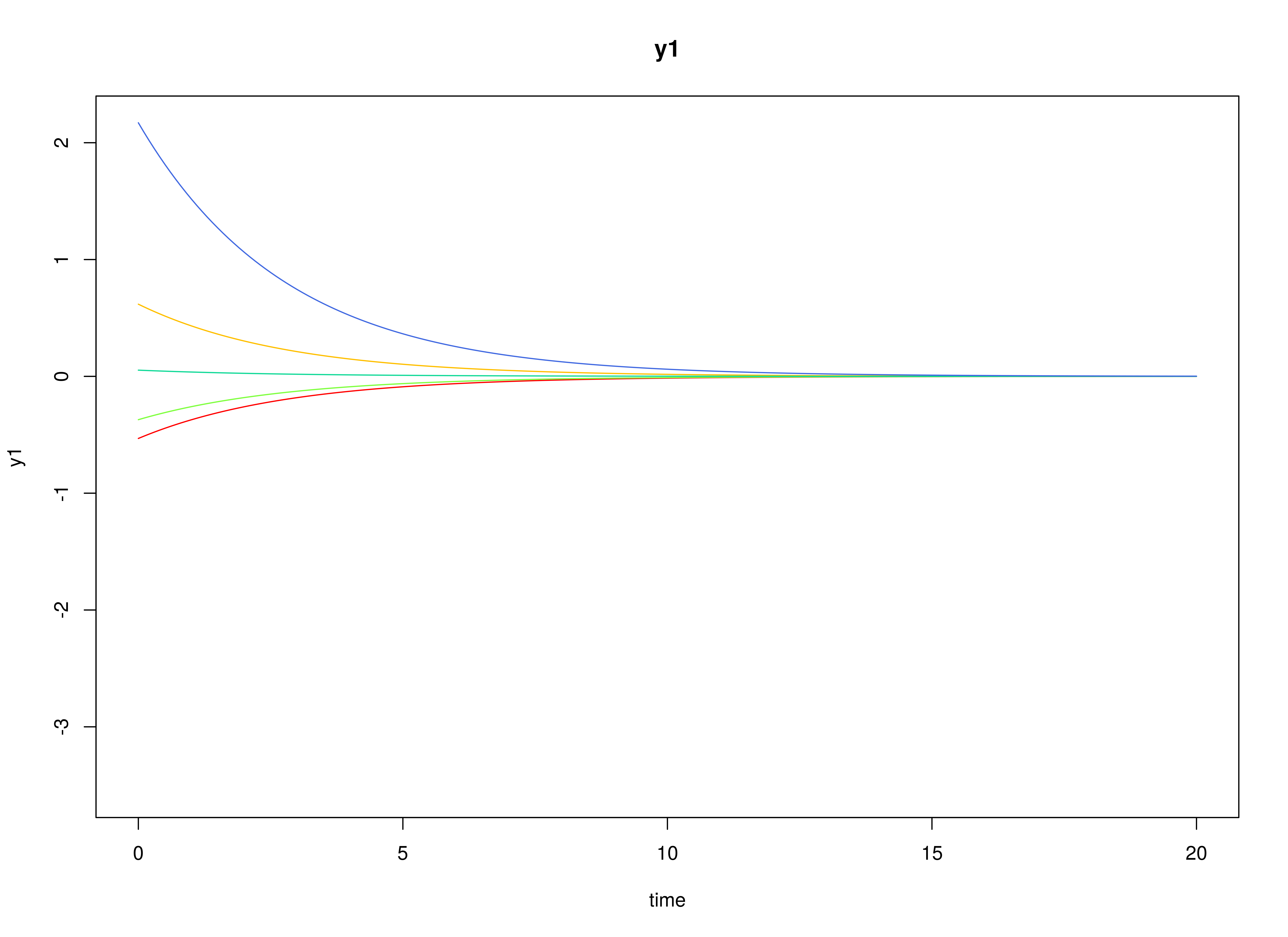
#> [3,] 0.0000000 0.0000000 0.4472136

Visualizing the Dynamics Without Measurement Error and Process Noise (n = 5 with Different Initial Condition)

Using the SimSSMOUFixed Function from the simStateSpace Package to Simulate Data

library(simStateSpace)
sim <- SimSSMOUFixed(
  n = n,
  time = time,
  delta_t = delta_t,
  mu0 = mu0,
  sigma0_l = sigma0_l,
  mu = mu,
  phi = phi,
  sigma_l = sigma_l,
  nu = nu,
  lambda = lambda,
  theta_l = theta_l,
  type = 0
)
data <- as.data.frame(sim)
head(data)
#>   id time          y1         y2         y3
#> 1  1  0.0  0.45047365 -1.2185550  0.6708638
#> 2  1  0.1 -0.84190461  0.1242594  0.1813493
#> 3  1  0.2  0.47289651 -0.2398710  0.5995107
#> 4  1  0.3  0.04089817 -0.6547109  0.4674929
#> 5  1  0.4 -1.37222946 -0.2010512 -0.3341885
#> 6  1  0.5 -0.62410106  0.5262251 -0.1892906
summary(data)
#>        id              time             y1                  y2           
#>  Min.   :   1.0   Min.   : 0.00   Min.   :-3.597165   Min.   :-4.091221  
#>  1st Qu.: 250.8   1st Qu.:24.98   1st Qu.:-0.487677   1st Qu.:-0.579974  
#>  Median : 500.5   Median :49.95   Median : 0.005842   Median : 0.009244  
#>  Mean   : 500.5   Mean   :49.95   Mean   : 0.005679   Mean   : 0.007098  
#>  3rd Qu.: 750.2   3rd Qu.:74.92   3rd Qu.: 0.500799   3rd Qu.: 0.595597  
#>  Max.   :1000.0   Max.   :99.90   Max.   : 3.447253   Max.   : 4.187849  
#>        y3           
#>  Min.   :-3.668061  
#>  1st Qu.:-0.474746  
#>  Median : 0.001988  
#>  Mean   : 0.001420  
#>  3rd Qu.: 0.477942  
#>  Max.   : 3.358401
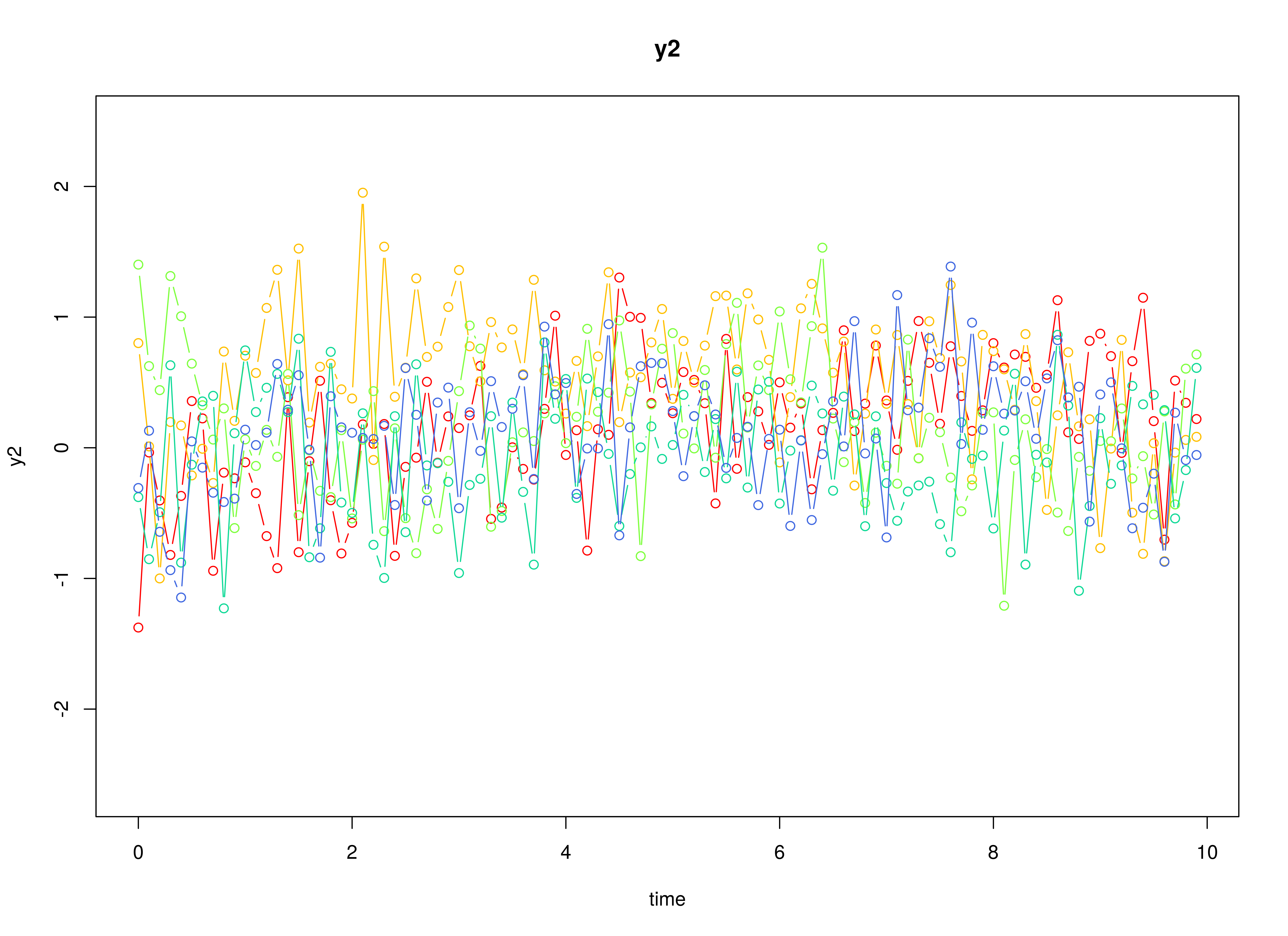
plot(sim)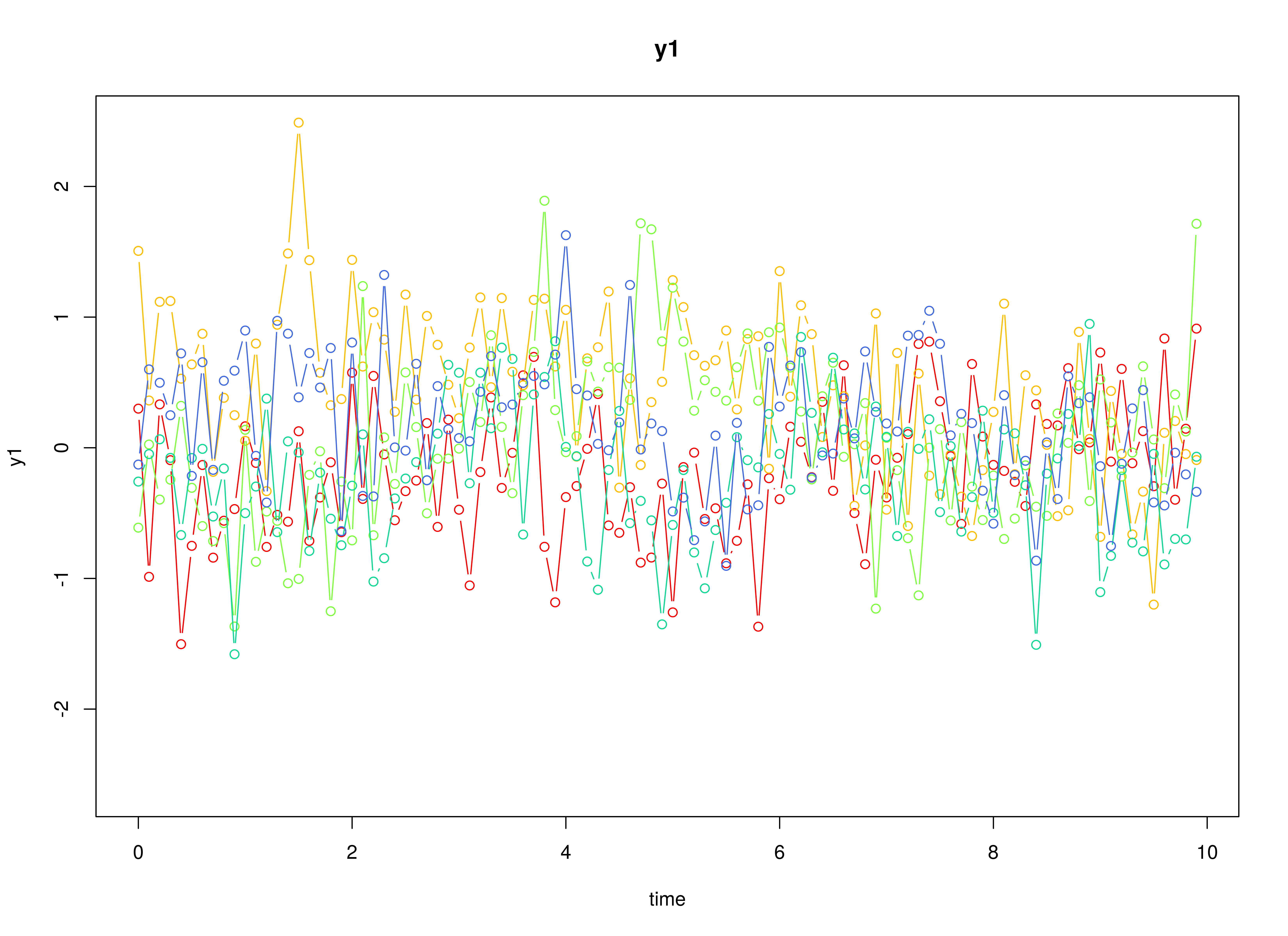

Model Fitting

Prepare Data

dynr_data <- dynr::dynr.data(
  dataframe = data,
  id = "id",
  time = "time",
  observed = c("y1", "y2", "y3")
)

Prepare Initial Condition

dynr_initial <- dynr::prep.initial(
  values.inistate = mu0,
  params.inistate = c("mu0_1_1", "mu0_2_1", "mu0_3_1"),
  values.inicov = sigma0,
  params.inicov = matrix(
    data = c(
      "sigma0_1_1", "sigma0_2_1", "sigma0_3_1",
      "sigma0_2_1", "sigma0_2_2", "sigma0_3_2",
      "sigma0_3_1", "sigma0_3_2", "sigma0_3_3"
    ),
    nrow = 3
  )
)

Prepare Measurement Model

dynr_measurement <- dynr::prep.measurement(
  values.load = diag(3),
  params.load = matrix(data = "fixed", nrow = 3, ncol = 3),
  state.names = c("eta_1", "eta_2", "eta_3"),
  obs.names = c("y1", "y2", "y3")
)

Prepare Dynamic Process

dynr_dynamics <- dynr::prep.formulaDynamics(
  formula = list(  
    eta_1 ~ (phi_1_1 * (eta_1 - mu_1_1)) + (phi_1_2 * (eta_2 - mu_2_1)) + (phi_1_3 * (eta_3 - mu_3_1)),
    eta_2 ~ (phi_2_1 * (eta_1 - mu_1_1)) + (phi_2_2 * (eta_2 - mu_2_1)) + (phi_2_3 * (eta_3 - mu_3_1)),
    eta_3 ~ (phi_3_1 * (eta_1 - mu_1_1)) + (phi_3_2 * (eta_2 - mu_2_1)) + (phi_3_3 * (eta_3 - mu_3_1))
  ),
  startval = c(
    mu_1_1 = mu[1], mu_2_1 = mu[2], mu_3_1 = mu[3],
    phi_1_1 = phi[1, 1], phi_1_2 = phi[1, 2], phi_1_3 = phi[1, 3],
    phi_2_1 = phi[2, 1], phi_2_2 = phi[2, 2], phi_2_3 = phi[2, 3],
    phi_3_1 = phi[3, 1], phi_3_2 = phi[3, 2], phi_3_3 = phi[3, 3]
  ),
  isContinuousTime = TRUE
)

Prepare Process Noise

dynr_noise <- dynr::prep.noise(
  values.latent = sigma,
  params.latent = matrix(
    data = c(
      "sigma_1_1", "sigma_2_1", "sigma_3_1",
      "sigma_2_1", "sigma_2_2", "sigma_3_2",
      "sigma_3_1", "sigma_3_2", "sigma_3_3"
    ),
    nrow = 3
  ),
  values.observed = theta,
  params.observed = matrix(
    data = c(
      "theta_1_1", "fixed", "fixed",
      "fixed", "theta_2_2", "fixed",
      "fixed", "fixed", "theta_3_3"
    ),
    nrow = 3
  )
)

Prepare the Model

model <- dynr::dynr.model(
  data = dynr_data,
  initial = dynr_initial,
  measurement = dynr_measurement,
  dynamics = dynr_dynamics,
  noise = dynr_noise,
  outfile = "ou.c"
)

Add lower and upper bounds to aid in the optimization.

model$lb[
  c(
    "phi_1_1",
    "phi_1_2",
    "phi_1_3",
    "phi_2_1",
    "phi_2_2",
    "phi_2_3",
    "phi_3_1",
    "phi_3_2",
    "phi_3_3"
  )
] <- -1.5
model$ub[
  c(
    "phi_1_1",
    "phi_1_2",
    "phi_1_3",
    "phi_2_1",
    "phi_2_2",
    "phi_2_3",
    "phi_3_1",
    "phi_3_2",
    "phi_3_3"
  )
] <- +1.5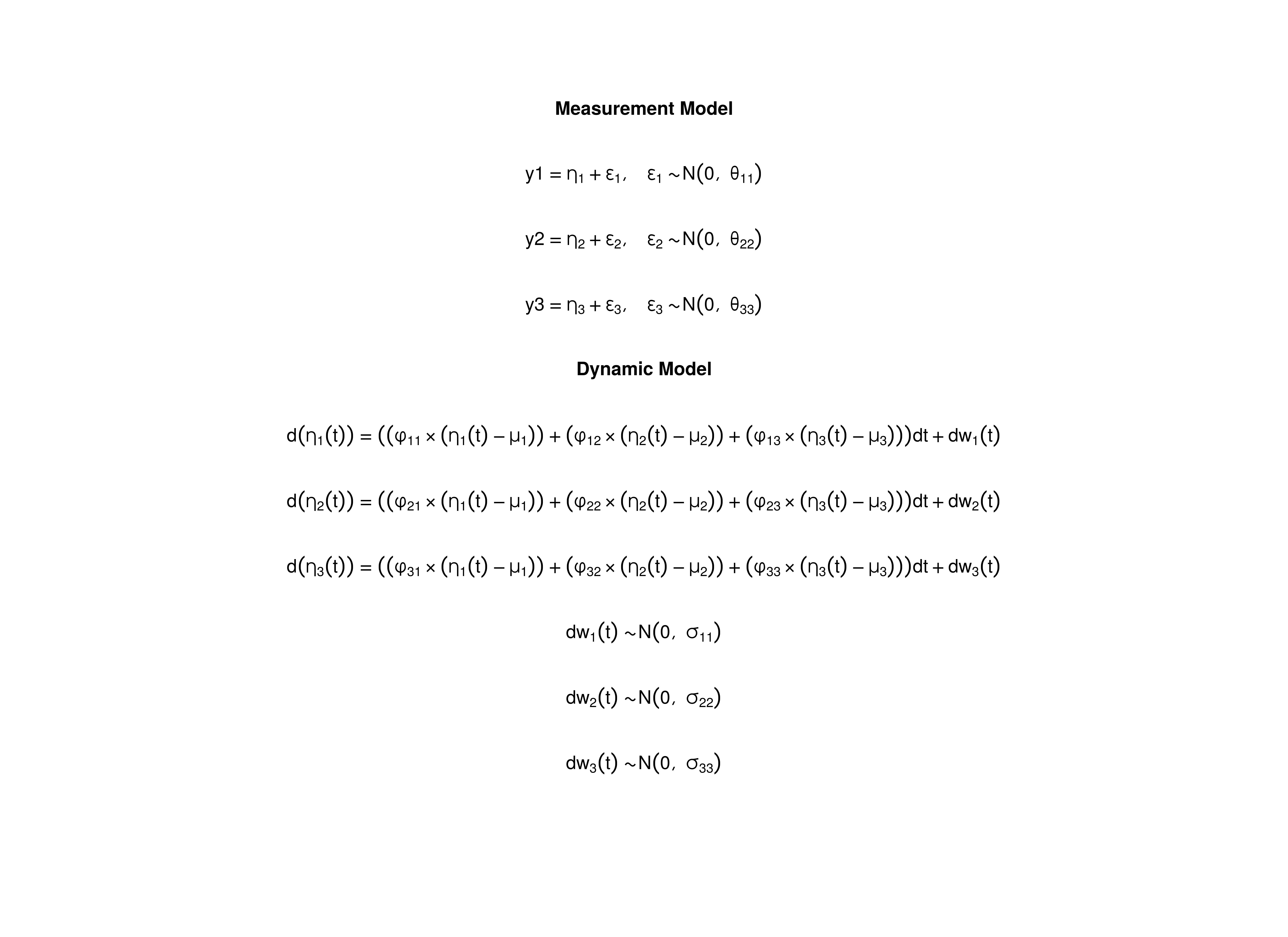

Fit the Model

results <- dynr::dynr.cook(
  model,
  debug_flag = TRUE,
  verbose = FALSE
)
#> [1] "Get ready!!!!"
#> using C compiler: ‘gcc (Ubuntu 13.3.0-6ubuntu2~24.04) 13.3.0’
#> Optimization function called.
#> Starting Hessian calculation ...
#> Finished Hessian calculation.
#> Original exit flag:  3 
#> Modified exit flag:  3 
#> Optimization terminated successfully: ftol_rel or ftol_abs was reached. 
#> Original fitted parameters:  0.004772387 0.006387041 0.001928491 -0.3583514 
#> -0.001773536 -0.0009242187 0.7717298 -0.5106306 -0.0009425439 -0.4504035 
#> 0.7272245 -0.6928862 -1.400091 0.09056937 -0.1990023 -2.655458 0.2825195 
#> -2.817898 -1.612043 -1.611921 -1.609778 -0.01930384 -0.001695005 0.002906709 
#> -1.098928 0.8660663 0.01750772 -1.302699 0.9128824 -2.284439 
#> 
#> Transformed fitted parameters:  0.004772387 0.006387041 0.001928491 -0.3583514 
#> -0.001773536 -0.0009242187 0.7717298 -0.5106306 -0.0009425439 -0.4504035 
#> 0.7272245 -0.6928862 0.2465745 0.0223321 -0.04906889 0.07228922 0.01540755 
#> 0.07510468 0.1994797 0.199504 0.199932 -0.01930384 -0.001695005 0.002906709 
#> 0.3332281 0.2885976 0.005834063 0.521742 0.2531716 0.3284367 
#> 
#> Doing end processing
#> Successful trial
#> Total Time: 20.74132 
#> Backend Time: 20.74114

Summary

summary(results)
#> Coefficients:
#>              Estimate Std. Error  t value   ci.lower   ci.upper Pr(>|t|)    
#> mu_1_1      0.0047724  0.0047757    0.999 -0.0045879  0.0141327    0.159    
#> mu_2_1      0.0063870  0.0077251    0.827 -0.0087539  0.0215280    0.204    
#> mu_3_1      0.0019285  0.0049565    0.389 -0.0077861  0.0116431    0.349    
#> phi_1_1    -0.3583514  0.0185105  -19.359 -0.3946314 -0.3220715   <2e-16 ***
#> phi_1_2    -0.0017735  0.0159471   -0.111 -0.0330293  0.0294823    0.456    
#> phi_1_3    -0.0009242  0.0114279   -0.081 -0.0233226  0.0214741    0.468    
#> phi_2_1     0.7717298  0.0094082   82.028  0.7532901  0.7901694   <2e-16 ***
#> phi_2_2    -0.5106306  0.0084223  -60.628 -0.5271381 -0.4941231   <2e-16 ***
#> phi_2_3    -0.0009425  0.0062797   -0.150 -0.0132505  0.0113655    0.440    
#> phi_3_1    -0.4504035  0.0081993  -54.932 -0.4664739 -0.4343332   <2e-16 ***
#> phi_3_2     0.7272245  0.0072519  100.280  0.7130110  0.7414380   <2e-16 ***
#> phi_3_3    -0.6928862  0.0055482 -124.886 -0.7037604 -0.6820119   <2e-16 ***
#> sigma_1_1   0.2465745  0.0031079   79.337  0.2404830  0.2526659   <2e-16 ***
#> sigma_2_1   0.0223321  0.0009036   24.714  0.0205610  0.0241032   <2e-16 ***
#> sigma_3_1  -0.0490689  0.0009402  -52.192 -0.0509116 -0.0472262   <2e-16 ***
#> sigma_2_2   0.0722892  0.0006781  106.606  0.0709602  0.0736183   <2e-16 ***
#> sigma_3_2   0.0154076  0.0004469   34.474  0.0145316  0.0162835   <2e-16 ***
#> sigma_3_3   0.0751047  0.0006930  108.377  0.0737464  0.0764629   <2e-16 ***
#> theta_1_1   0.1994797  0.0004123  483.818  0.1986716  0.2002878   <2e-16 ***
#> theta_2_2   0.1995040  0.0003204  622.761  0.1988761  0.2001319   <2e-16 ***
#> theta_3_3   0.1999320  0.0003213  622.319  0.1993023  0.2005617   <2e-16 ***
#> mu0_1_1    -0.0193038  0.0215547   -0.896 -0.0615503  0.0229426    0.185    
#> mu0_2_1    -0.0016950  0.0369205   -0.046 -0.0740579  0.0706679    0.482    
#> mu0_3_1     0.0029067  0.0345815    0.084 -0.0648718  0.0706852    0.467    
#> sigma0_1_1  0.3332281  0.0254503   13.093  0.2833463  0.3831098   <2e-16 ***
#> sigma0_2_1  0.2885976  0.0321793    8.968  0.2255274  0.3516678   <2e-16 ***
#> sigma0_3_1  0.0058341  0.0218162    0.267 -0.0369249  0.0485930    0.395    
#> sigma0_2_2  0.5217420  0.0553415    9.428  0.4132746  0.6302093   <2e-16 ***
#> sigma0_3_2  0.2531716  0.0311815    8.119  0.1920571  0.3142862   <2e-16 ***
#> sigma0_3_3  0.3284367  0.0303100   10.836  0.2690302  0.3878433   <2e-16 ***
#> ---
#> Signif. codes:  0 '***' 0.001 '**' 0.01 '*' 0.05 '.' 0.1 ' ' 1
#> 
#> -2 log-likelihood value at convergence = 4293422.48
#> AIC = 4293482.48
#> BIC = 4293836.94

#> [1] -0.019303838 -0.001695005  0.002906709

Parameter Estimates

mu_hat
#> [1] 0.004772387 0.006387041 0.001928491
phi_hat
#>            [,1]         [,2]          [,3]
#> [1,] -0.3583514 -0.001773536 -0.0009242187
#> [2,]  0.7717298 -0.510630602 -0.0009425439
#> [3,] -0.4504035  0.727224464 -0.6928861600
sigma_hat
#>             [,1]       [,2]        [,3]
#> [1,]  0.24657448 0.02233210 -0.04906889
#> [2,]  0.02233210 0.07228922  0.01540755
#> [3,] -0.04906889 0.01540755  0.07510468
theta_hat
#>           [,1]     [,2]     [,3]
#> [1,] 0.1994797 0.000000 0.000000
#> [2,] 0.0000000 0.199504 0.000000
#> [3,] 0.0000000 0.000000 0.199932
mu0_hat
#> [1] -0.019303838 -0.001695005  0.002906709
sigma0_hat
#>             [,1]      [,2]        [,3]
#> [1,] 0.333228051 0.2885976 0.005834063
#> [2,] 0.288597597 0.5217420 0.253171644
#> [3,] 0.005834063 0.2531716 0.328436733
beta_var1_hat <- expm::expm(phi_hat)
beta_var1_hat
#>            [,1]         [,2]          [,3]
#> [1,]  0.6984495 -0.001349417 -0.0005482773
#> [2,]  0.5002334  0.599439403 -0.0007292751
#> [3,] -0.1003474  0.399072761  0.5000156072

References

Chow, S.-M., Ho, M. R., Hamaker, E. L., & Dolan, C. V. (2010). Equivalence and differences between structural equation modeling and state-space modeling techniques. Structural Equation Modeling: A Multidisciplinary Journal, 17(2), 303–332. https://doi.org/10.1080/10705511003661553

Chow, S.-M., Losardo, D., Park, J., & Molenaar, P. C. M. (2023). Continuous-time dynamic models: Connections to structural equation models and other discrete-time models. In R. H. Hoyle (Ed.), Handbook of structural equation modeling (2nd ed.). The Guilford Press.

Deboeck, P. R., & Preacher, K. J. (2015). No need to be discrete: A method for continuous time mediation analysis. Structural Equation Modeling: A Multidisciplinary Journal, 23(1), 61–75. https://doi.org/10.1080/10705511.2014.973960

Oravecz, Z., Tuerlinckx, F., & Vandekerckhove, J. (2011). A hierarchical latent stochastic differential equation model for affective dynamics. Psychological Methods, 16(4), 468–490. https://doi.org/10.1037/a0024375

Ou, L., Hunter, M. D., & Chow, S.-M. (2019). What’s for dynr: A package for linear and nonlinear dynamic modeling in R. The R Journal, 11(1), 91. https://doi.org/10.32614/rj-2019-012

R Core Team. (2024). R: A language and environment for statistical computing. R Foundation for Statistical Computing. https://www.R-project.org/

Uhlenbeck, G. E., & Ornstein, L. S. (1930). On the theory of the brownian motion. Physical Review, 36(5), 823–841. https://doi.org/10.1103/physrev.36.823