Meta-Analysis of Continuous-Time Vector Autoregressive Model Estimates

Dynamics Description

The Stable Reciprocal Regulation process is modeled as a continuous-time bivariate dynamic system in which two latent psychological constructs (e.g., negative and positive affect) mutually influence each other through their instantaneous rates of change. The dynamics are governed by the continuous-time drift matrix whose negative diagonal elements indicate substantial self-regulation: deviations from a person’s equilibrium are pulled back toward baseline at a moderate-to-strong rate. The negative off-diagonal elements reflect reciprocal inhibition: higher levels of one construct are associated with an increased instantaneous tendency for the other construct to decline. Because the cross-effects are modest relative to the self-regulatory terms, the system exhibits stable, non-oscillatory relaxation back toward person-specific equilibrium points.

Individuals are allowed to differ in both their self-regulatory rates and the strength of these antagonistic couplings. Stochastic disturbances enter through the process-noise covariance, permitting small (potentially correlated) departures from the deterministic drift, while measurement errors are assumed to be minimal and comparable across indicators. Overall, this pattern captures a psychologically plausible mechanism of reciprocal inhibition in which short-term perturbations in one component (e.g., negative affect) are naturally counteracted by compensatory adjustment in the other (e.g., positive affect), supporting emotional homeostasis over time.

Model

The measurement model is given by $\begin{equation} \mathbf{y}_{i, t} = \boldsymbol{\eta}_{i, t} \end{equation}$ where $\mathbf{y}_{i, t}$ and $\boldsymbol{\eta}_{i, t}$ are random variables.

The dynamic structure is given by $\begin{equation} \mathrm{d} \boldsymbol{\eta}_{i, t} = \left( \boldsymbol{\alpha}_{i} + \boldsymbol{\beta}_{i} \boldsymbol{\eta}_{i, t} \right) \mathrm{d} t + \boldsymbol{\Psi}^{\frac{1}{2}} \mathrm{d} \mathbf{W}_{i, t} \end{equation}$ where $\mathrm{d}\boldsymbol{W}_{i, t}$ is a Wiener process or Brownian motion, which represents random fluctuations, $\boldsymbol{\eta}_{i, t}$ is a random variable, and $\boldsymbol{\beta}_{i}$ , and $\boldsymbol{\Psi}$ are model parameters. Here, $\boldsymbol{\eta}_{i, t}$ is a vector of latent variables at time $t$ and individual $i$ . $\boldsymbol{\beta}_{i}$ is a matrix of auto and cross effect coefficients for individual $i$ , and $\boldsymbol{\Psi}$ the covariance matrix of the process noise.

Alternative Parameterization

An alternative parameterization of the dynamic structure that directly estimates the set point vector $\boldsymbol{\mu}_{i}$ is given by $\begin{equation} \mathrm{d} \boldsymbol{\eta}_{i, t} = \boldsymbol{\beta}_{i} \left( \boldsymbol{\eta}_{i, t} - \boldsymbol{\mu}_{i} \right) \mathrm{d} t + \boldsymbol{\Psi}^{\frac{1}{2}} \mathrm{d} \mathbf{W}_{i, t} . \end{equation}$

Algebraic manipulation of the equation results in the following $\begin{equation} \mathrm{d} \boldsymbol{\eta}_{i, t} = \left( - \boldsymbol{\beta}_{i} \boldsymbol{\mu}_{i} + \boldsymbol{\beta}_{i} \boldsymbol{\eta}_{i, t} \right) \mathrm{d} t + \boldsymbol{\Psi}^{\frac{1}{2}} \mathrm{d} \mathbf{W}_{i, t} \end{equation}$ where we can see that the intercept vector $\boldsymbol{\alpha}_{i}$ is implied by $- \boldsymbol{\beta}_{i} \boldsymbol{\mu}_{i}$ .

Data Generation

Notation

Let $t = 1000$ be the number of time points and $n = 100$ be the number of individuals.

Let the initial condition $\boldsymbol{\eta}_{0}$ be given by $\begin{equation} \boldsymbol{\eta}_{0} \sim \mathcal{N} \left( \boldsymbol{\mu}_{\boldsymbol{\eta} \mid 0}, \boldsymbol{\Sigma}_{\boldsymbol{\eta} \mid 0} \right) . \end{equation}$ $\boldsymbol{\mu}_{\boldsymbol{\eta} \mid 0}$ and $\boldsymbol{\Sigma}_{\boldsymbol{\eta} \mid 0}$ are functions of $\boldsymbol{\alpha}$ and $\boldsymbol{\beta}$ .

Let the set point vector $\boldsymbol{\mu}$ be normally distributed with the following means $\begin{equation} \left( \begin{array}{c} 2.87 \\ 2.04 \\ \end{array} \right) \end{equation}$ and covariance matrix $\begin{equation} \left( \begin{array}{cc} 1.2 & 0.46 \\ 0.46 & 1.1 \\ \end{array} \right) . \end{equation}$

Let the transition matrix $\boldsymbol{\beta}$ be normally distributed with the following means $\begin{equation} \left( \begin{array}{cc} -1.2843504 & -0.1792463 \\ -0.1307004 & -1.3590363 \\ \end{array} \right) \end{equation}$ and covariance matrix $\begin{equation} \left( \begin{array}{cccc} 0.017 & 0.005 & 0.001 & 0.008 \\ 0.005 & 0.008 & 0.001 & 0.006 \\ 0.001 & 0.001 & 0.001 & 0.002 \\ 0.008 & 0.006 & 0.002 & 0.026 \\ \end{array} \right) . \end{equation}$

The SimMuN and SimPhiN functions from the simStateSpace package generate random set point vectors and drift matrices from the multivariate normal distribution. Note that the SimPhiN function generates drift matrices that are weakly stationary with an option to set lower and upper bounds.

Let the dynamic process noise $\boldsymbol{\Psi}$ be given by $\begin{equation} \boldsymbol{\Psi} = \left( \begin{array}{cc} 1.3 & 0.57 \\ 0.57 & 1.56 \\ \end{array} \right) . \end{equation}$

R Function Arguments

n
#> [1] 100
time
#> [1] 1000
# first mu0 in the list of length n
mu0[[1]]
#> [1] 2.287769 2.606098
# first sigma0 in the list of length n
sigma0[[1]]
#>           [,1]      [,2]
#> [1,] 0.5037766 0.1478276
#> [2,] 0.1478276 0.5694164
# first sigma0_l in the list of length n
sigma0_l[[1]] # sigma0_l <- t(chol(sigma0))
#>           [,1]      [,2]
#> [1,] 0.7097722 0.0000000
#> [2,] 0.2082747 0.7252848
# first alpha in the list of length n
alpha[[1]]
#> [1] 3.312112 3.842713
# first beta in the list of length n
beta[[1]]
#>           [,1]      [,2]
#> [1,] -1.235608 -0.186227
#> [2,] -0.169327 -1.325864
# first psi in the list of length n
psi[[1]]
#>      [,1] [,2]
#> [1,] 1.30 0.57
#> [2,] 0.57 1.56
psi_l[[1]] # psi_l <- t(chol(psi))
#>           [,1]     [,2]
#> [1,] 1.1401754 0.000000
#> [2,] 0.4999231 1.144586
# first mu (set point) in the list of length n
mu[[1]]
#> [1] 2.287769 2.606098

Visualizing the Dynamics Without Process Noise and Measurement Error (n = 5 with Different Initial Condition)

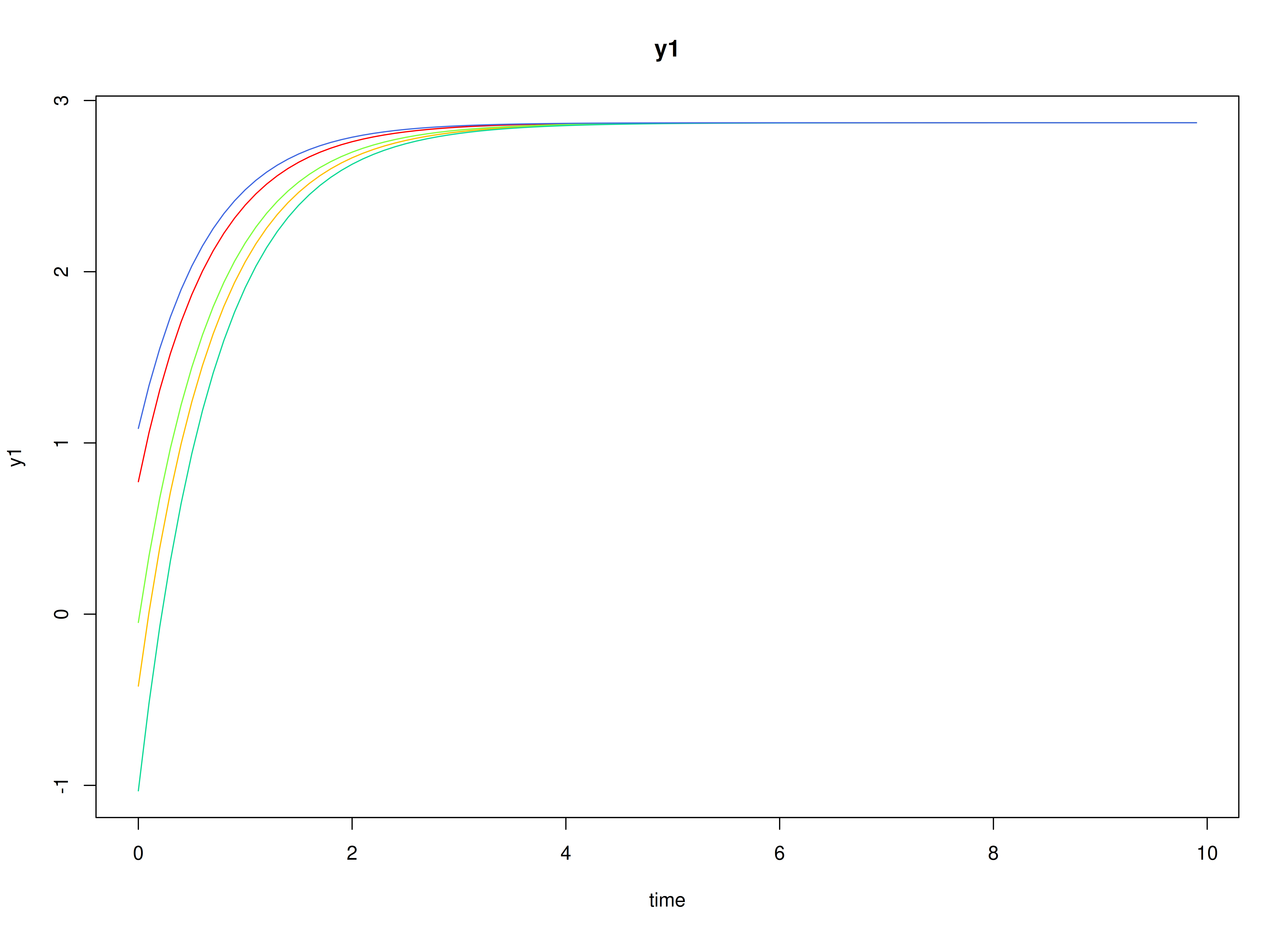
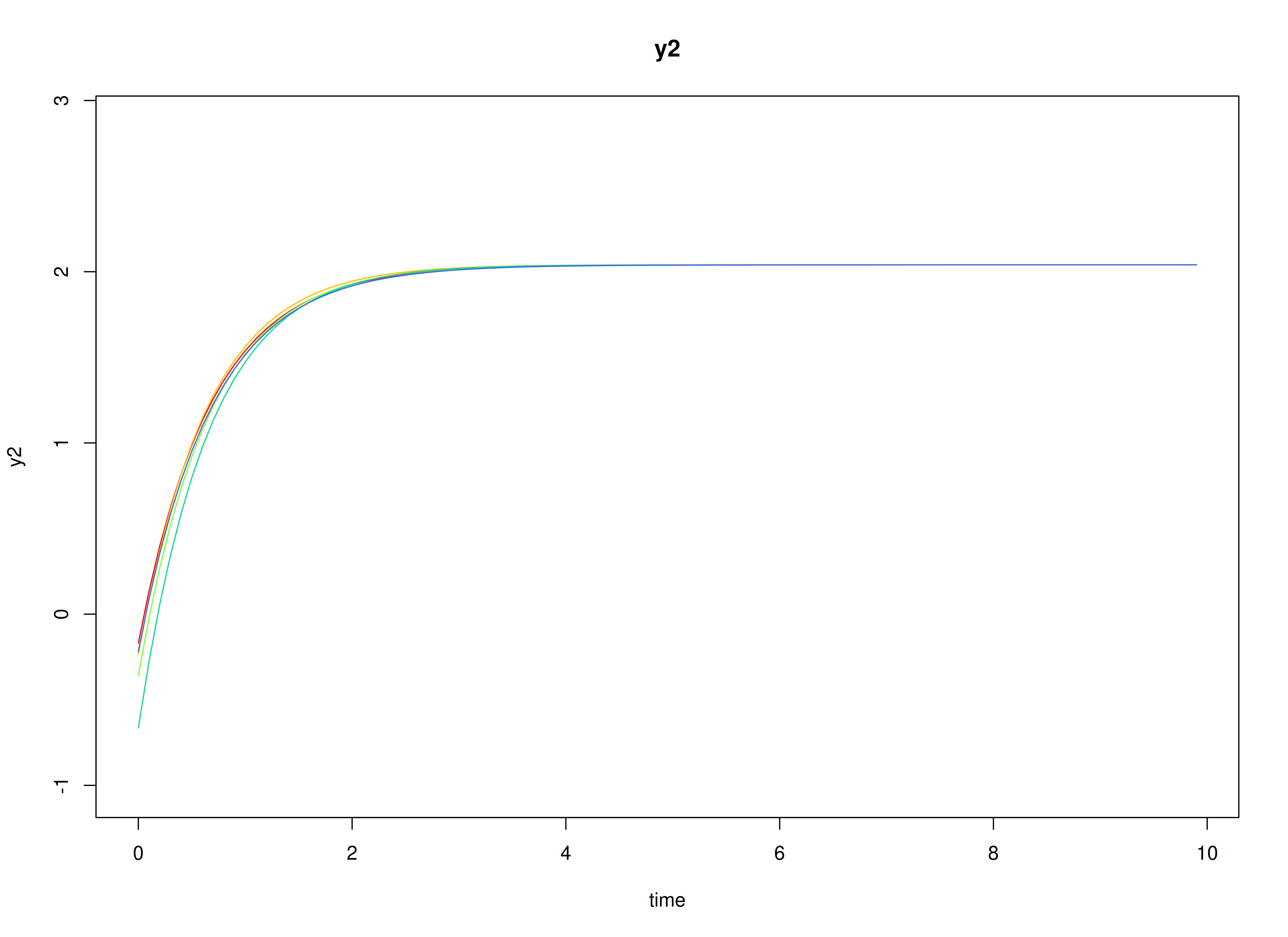
Using the `SimSSMLinSDEFixed` Function from the `simStateSpace` Package to Simulate Data

Note: The SimSSMLinSDEFixed function uses a different set of parameter names. See help(SimSSMLinSDEFixed) for more details.

library(simStateSpace)
sim <- SimSSMLinSDEIVary(
  n = n,
  time = time,
  delta_t = 0.1,
  mu0 = mu0,
  sigma0_l = sigma0_l,
  iota = alpha,
  phi = beta,
  sigma_l = psi_l,
  nu = nu,
  lambda = lambda,
  theta_l = theta_l
)
data <- as.data.frame(sim)
head(data)
#>   id time       y1       y2
#> 1  1  0.0 2.523315 3.353060
#> 2  1  0.1 2.309397 3.020899
#> 3  1  0.2 2.600318 3.078564
#> 4  1  0.3 2.698363 2.929001
#> 5  1  0.4 2.444623 2.861375
#> 6  1  0.5 3.190602 2.891174
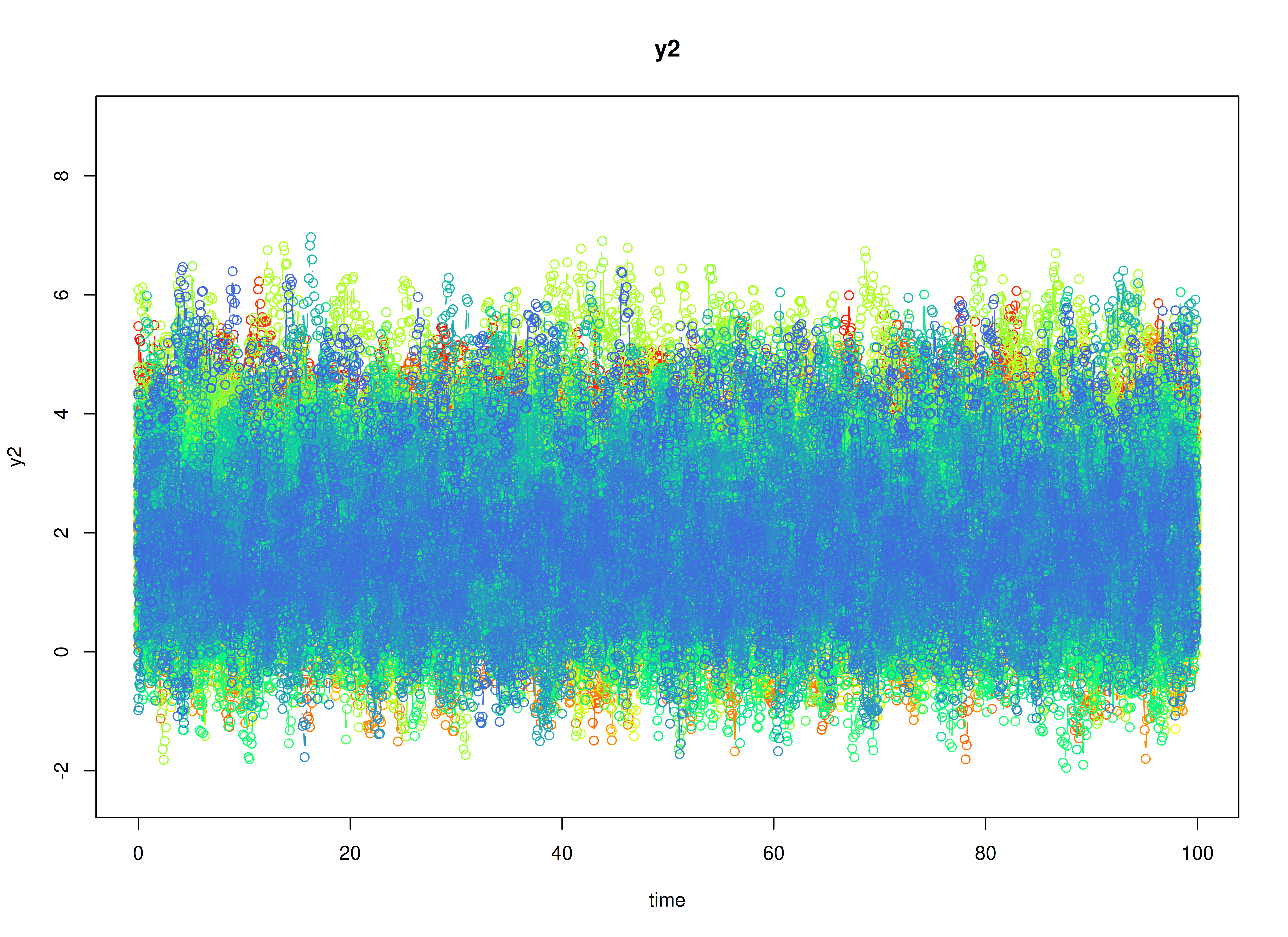
summary(data)
#>        id              time             y1               y2        
#>  Min.   :  1.00   Min.   : 0.00   Min.   :-2.335   Min.   :-1.951  
#>  1st Qu.: 25.75   1st Qu.:24.98   1st Qu.: 2.093   1st Qu.: 1.261  
#>  Median : 50.50   Median :49.95   Median : 2.990   Median : 2.187  
#>  Mean   : 50.50   Mean   :49.95   Mean   : 2.975   Mean   : 2.185  
#>  3rd Qu.: 75.25   3rd Qu.:74.92   3rd Qu.: 3.873   3rd Qu.: 3.081  
#>  Max.   :100.00   Max.   :99.90   Max.   : 8.893   Max.   : 6.970
plot(sim)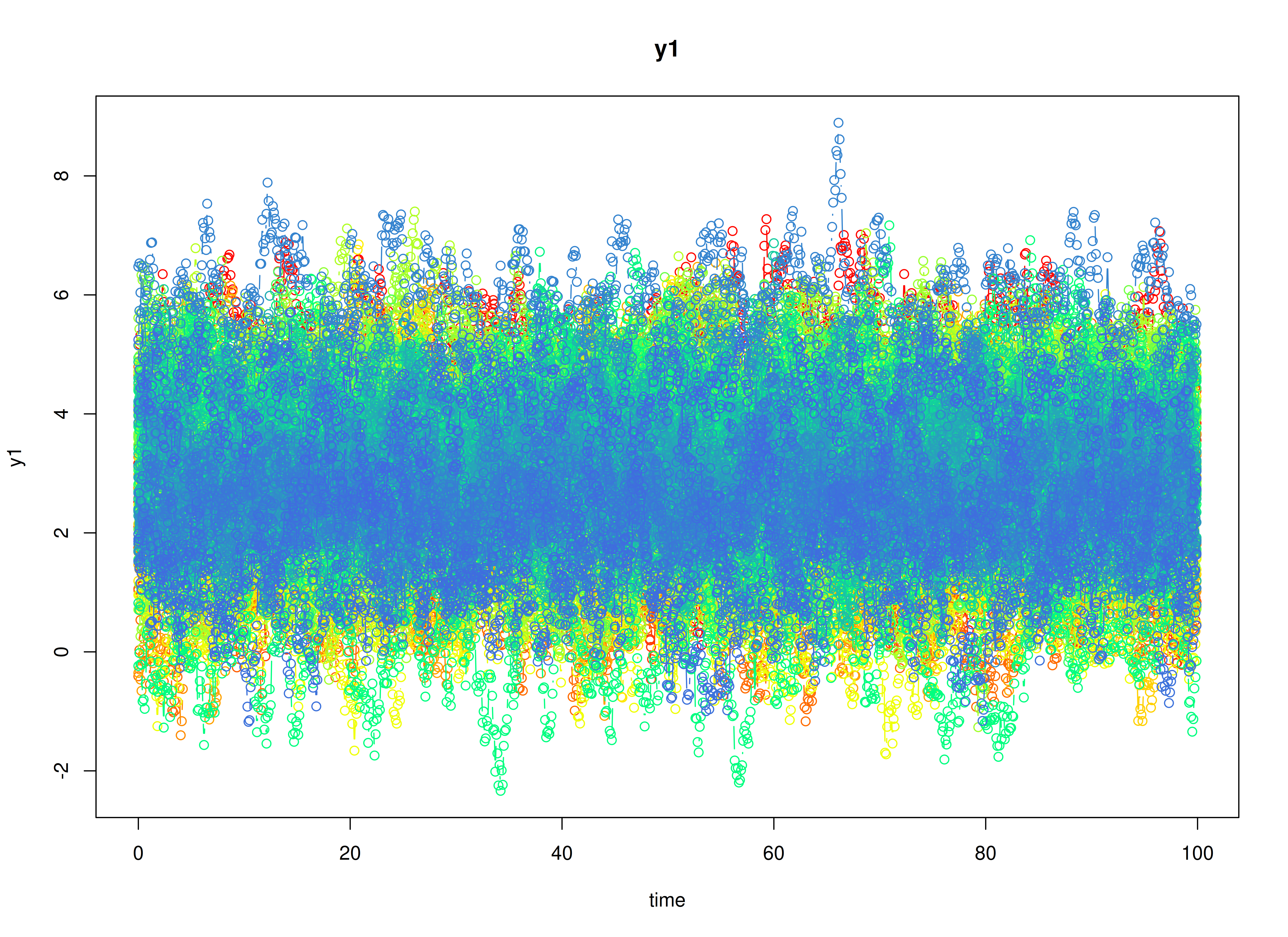

Stage 1: Person-Specific VAR Model

library(OpenMx)
library(fitVARMxID)

The FitVARMxID function fits a VAR model on each individual $i$ .

Note: Consider using the argument ncores to use multiple cores for parallel processing.

fit <- FitVARMxID(
  data = data,
  observed = c("y1", "y2"),
  id = "id",
  ct = TRUE,
  time = "time",
  center = TRUE,
  ncores = parallel::detectCores()
)

summary(
  fit,
  means = TRUE
)
#> Call:
#> FitVARMxID(data = data, observed = c("y1", "y2"), id = "id", 
#>     time = "time", ct = TRUE, center = TRUE, ncores = parallel::detectCores())
#> 
#> Convergence:
#> 100.0%
#> 
#> Means of the estimated paramaters per individual.
#>   mu[1,1]   mu[2,1] beta[1,1] beta[2,1] beta[1,2] beta[2,2]  psi[1,1]  psi[2,1] 
#>    2.9743    2.1847   -1.3528   -0.1673   -0.1959   -1.4373    1.3040    0.5685 
#>  psi[2,2] 
#>    1.5566

Stage 2: Random-Effects Meta-Analysis of Person-Specific Set Points and Dynamics

We synthesize the person-specific estimates to recover population-level effects and their between-person variability. We use a random-effects model so the pooled mean reflects both within-person estimation uncertainty and between-person heterogeneity.

All available parameters are meta-analyzed by default. Setting cov_dyn = FALSE, meta-analyzes only the set points and drift matrix. Setting tau_sqr_l_free, such that covariances between mu and beta are constained to zero, simplifies the random effects.

tau_sqr_l_free <- matrix(
  data = c(
    FALSE, FALSE, FALSE, FALSE, FALSE, FALSE,
    TRUE, FALSE, FALSE, FALSE, FALSE, FALSE,
    FALSE, FALSE, FALSE, FALSE, FALSE, FALSE,
    FALSE, FALSE, TRUE, FALSE, FALSE, FALSE,
    FALSE, FALSE, TRUE, TRUE, FALSE, FALSE,
    FALSE, FALSE, TRUE, TRUE, TRUE, FALSE
  ),
  byrow = TRUE,
  nrow = 6,
  ncol = 6
)
# FALSE values in tau_sqr_l_free will be treated as fixed values.
# TRUE values in tau_sqr_l_free will be treated as starting values.
tau_sqr_l_values <- matrix(
  data = 0,
  nrow = 6,
  ncol = 6
)

Note: Consider using the argument ncores to use multiple cores for parallel processing.

library(metaDyn)
metavar <- MetaVARMx(
  object = fit,
  tau_sqr_l_free = tau_sqr_l_free,
  tau_sqr_l_values = tau_sqr_l_values,
  cov_dyn = FALSE,
  ncores = parallel::detectCores()
)

summary(metavar)
#> Call:
#> MetaVARMx(object = fit, tau_sqr_l_free = tau_sqr_l_free, tau_sqr_l_values = tau_sqr_l_values, 
#>     cov_dyn = FALSE, ncores = parallel::detectCores())
#> 
#> Status code:
#> 0
#> 
#> CI type:
#> "normal"
#> 
#>                  est     se         z      p    2.5%   97.5%
#> alpha[1,1]    2.9742 0.1120   26.5553 0.0000  2.7547  3.1937
#> alpha[2,1]    2.1845 0.1062   20.5783 0.0000  1.9765  2.3926
#> alpha[3,1]   -1.3129 0.0238  -55.2242 0.0000 -1.3595 -1.2663
#> alpha[4,1]   -0.1670 0.0225   -7.4221 0.0000 -0.2111 -0.1229
#> alpha[5,1]   -0.1943 0.0186  -10.4597 0.0000 -0.2307 -0.1579
#> alpha[6,1]   -1.3984 0.0251  -55.8086 0.0000 -1.4475 -1.3492
#> tau_sqr[1,1]  1.2471 0.1775    7.0246 0.0000  0.8991  1.5950
#> tau_sqr[2,1]  0.5434 0.1307    4.1583 0.0000  0.2873  0.7996
#> tau_sqr[2,2]  1.1190 0.1593    7.0232 0.0000  0.8067  1.4313
#> tau_sqr[3,3]  0.0209 0.0072    2.8945 0.0038  0.0067  0.0350
#> tau_sqr[4,3]  0.0013 0.0048    0.2586 0.7959 -0.0082  0.0108
#> tau_sqr[5,3]  0.0005 0.0041    0.1170 0.9069 -0.0075  0.0084
#> tau_sqr[6,3] -0.0046 0.0058   -0.7892 0.4300 -0.0159  0.0068
#> tau_sqr[4,4]  0.0088 0.0063    1.3986 0.1619 -0.0035  0.0212
#> tau_sqr[5,4]  0.0045 0.0032    1.4267 0.1537 -0.0017  0.0108
#> tau_sqr[6,4] -0.0038 0.0056   -0.6877 0.4916 -0.0147  0.0071
#> tau_sqr[5,5]  0.0035 0.0036    0.9680 0.3330 -0.0036  0.0106
#> tau_sqr[6,5]  0.0032 0.0042    0.7698 0.4414 -0.0050  0.0114
#> tau_sqr[6,6]  0.0251 0.0079    3.1574 0.0016  0.0095  0.0406
#> i_sqr[1,1]    0.9950 0.0007 1397.5277 0.0000  0.9936  0.9964
#> i_sqr[2,1]    0.9932 0.0010 1034.5138 0.0000  0.9913  0.9951
#> i_sqr[3,1]    0.3866 0.0819    4.7197 0.0000  0.2260  0.5471
#> i_sqr[4,1]    0.2614 0.1046    2.4981 0.0125  0.0563  0.4664
#> i_sqr[5,1]    0.1538 0.1049    1.4661 0.1426 -0.0518  0.3594
#> i_sqr[6,1]    0.4421 0.0735    6.0149 0.0000  0.2981  0.5862

Normal Theory Confidence Intervals

confint(metavar, level = 0.95)
#>                     2.5 %       97.5 %
#> alpha[1,1]    2.754697920  3.193733175
#> alpha[2,1]    1.976480275  2.392610565
#> alpha[3,1]   -1.359474981 -1.266284141
#> alpha[4,1]   -0.211132346 -0.122918630
#> alpha[5,1]   -0.230690233 -0.157879112
#> alpha[6,1]   -1.447460395 -1.349241914
#> tau_sqr[1,1]  0.899135556  1.595042757
#> tau_sqr[2,1]  0.287298520  0.799593547
#> tau_sqr[2,2]  0.806737218  1.431303262
#> tau_sqr[3,3]  0.006747421  0.035049670
#> tau_sqr[4,3] -0.008248909  0.010756532
#> tau_sqr[5,3] -0.007494722  0.008446156
#> tau_sqr[6,3] -0.015888876  0.006766169
#> tau_sqr[4,4] -0.003547420  0.021224104
#> tau_sqr[5,4] -0.001693146  0.010753552
#> tau_sqr[6,4] -0.014733930  0.007079880
#> tau_sqr[5,5] -0.003582845  0.010575514
#> tau_sqr[6,5] -0.004985040  0.011433547
#> tau_sqr[6,6]  0.009510610  0.040645736
#> i_sqr[1,1]    0.993578025  0.996368828
#> i_sqr[2,1]    0.991335998  0.995099449
#> i_sqr[3,1]    0.226027843  0.547081391
#> i_sqr[4,1]    0.056303462  0.466432631
#> i_sqr[5,1]   -0.051801426  0.359393016
#> i_sqr[6,1]    0.298060935  0.586200280

confint(metavar, level = 0.99)
#>                     0.5 %      99.5 %
#> alpha[1,1]    2.685720483  3.26271061
#> alpha[2,1]    1.911101468  2.45798937
#> alpha[3,1]   -1.374116323 -1.25164280
#> alpha[4,1]   -0.224991725 -0.10905925
#> alpha[5,1]   -0.242129689 -0.14643966
#> alpha[6,1]   -1.462891636 -1.33381067
#> tau_sqr[1,1]  0.789800611  1.70437770
#> tau_sqr[2,1]  0.206811138  0.88008093
#> tau_sqr[2,2]  0.708610781  1.52942970
#> tau_sqr[3,3]  0.002300815  0.03949628
#> tau_sqr[4,3] -0.011234880  0.01374250
#> tau_sqr[5,3] -0.009999215  0.01095065
#> tau_sqr[6,3] -0.019448242  0.01032553
#> tau_sqr[4,4] -0.007439309  0.02511599
#> tau_sqr[5,4] -0.003648663  0.01270907
#> tau_sqr[6,4] -0.018161128  0.01050708
#> tau_sqr[5,5] -0.005807285  0.01279995
#> tau_sqr[6,5] -0.007564587  0.01401309
#> tau_sqr[6,6]  0.004618928  0.04553742
#> i_sqr[1,1]    0.993139558  0.99680729
#> i_sqr[2,1]    0.990744718  0.99569073
#> i_sqr[3,1]    0.175586675  0.59752256
#> i_sqr[4,1]   -0.008132500  0.53086859
#> i_sqr[5,1]   -0.116404755  0.42399634
#> i_sqr[6,1]    0.252790963  0.63147025

Robust Confidence Intervals

confint(metavar, level = 0.95, robust = TRUE)
#>                     2.5 %       97.5 %
#> alpha[1,1]    2.753595167  3.194835928
#> alpha[2,1]    1.975427810  2.393663029
#> alpha[3,1]   -1.358281426 -1.267477696
#> alpha[4,1]   -0.211854456 -0.122196521
#> alpha[5,1]   -0.230839452 -0.157729893
#> alpha[6,1]   -1.445575820 -1.351126489
#> tau_sqr[1,1]  0.908528628  1.585649685
#> tau_sqr[2,1]  0.284665842  0.802226224
#> tau_sqr[2,2]  0.848743506  1.389296975
#> tau_sqr[3,3]  0.006102537  0.035694554
#> tau_sqr[4,3] -0.007485709  0.009993332
#> tau_sqr[5,3] -0.007525424  0.008476859
#> tau_sqr[6,3] -0.015341374  0.006218667
#> tau_sqr[4,4] -0.002283607  0.019960290
#> tau_sqr[5,4] -0.001047066  0.010107472
#> tau_sqr[6,4] -0.012836700  0.005182651
#> tau_sqr[5,5] -0.002928275  0.009920944
#> tau_sqr[6,5] -0.004278437  0.010726945
#> tau_sqr[6,6]  0.005258147  0.044898199
#> i_sqr[1,1]    0.993615694  0.996331158
#> i_sqr[2,1]    0.991608488  0.994826960
#> i_sqr[3,1]    0.218712000  0.554397234
#> i_sqr[4,1]    0.072856492  0.449879601
#> i_sqr[5,1]   -0.024244107  0.331835696
#> i_sqr[6,1]    0.226365579  0.657895637

confint(metavar, level = 0.99, robust = TRUE)
#>                      0.5 %       99.5 %
#> alpha[1,1]    2.6842712195  3.264159876
#> alpha[2,1]    1.9097182949  2.459372544
#> alpha[3,1]   -1.3725477260 -1.253211396
#> alpha[4,1]   -0.2259407384 -0.108110238
#> alpha[5,1]   -0.2423257958 -0.146243549
#> alpha[6,1]   -1.4604148850 -1.336287424
#> tau_sqr[1,1]  0.8021451999  1.692033113
#> tau_sqr[2,1]  0.2033512131  0.883540853
#> tau_sqr[2,2]  0.7638164007  1.474224080
#> tau_sqr[3,3]  0.0014532938  0.040343797
#> tau_sqr[4,3] -0.0102318653  0.012739489
#> tau_sqr[5,3] -0.0100395653  0.010991000
#> tau_sqr[6,3] -0.0187287022  0.009605995
#> tau_sqr[4,4] -0.0057783762  0.023455060
#> tau_sqr[5,4] -0.0027995706  0.011859977
#> tau_sqr[6,4] -0.0156677456  0.008013696
#> tau_sqr[5,5] -0.0049470337  0.011939703
#> tau_sqr[6,5] -0.0066359535  0.013084461
#> tau_sqr[6,6] -0.0009697561  0.051126102
#> i_sqr[1,1]    0.9931890636  0.996757789
#> i_sqr[2,1]    0.9911028290  0.995332619
#> i_sqr[3,1]    0.1659720271  0.607137207
#> i_sqr[4,1]    0.0136218691  0.509114224
#> i_sqr[5,1]   -0.0801882983  0.387779888
#> i_sqr[6,1]    0.1585672927  0.725693922

The fixed part of the random-effects model gives pooled means $\boldsymbol{\alpha} = \mathbb{E} \left[ \mathrm{Vec} \left( \boldsymbol{\mu}, \boldsymbol{\beta} \right) \right]$ .
The random part yields between-person covariances ( $\boldsymbol{\tau}^{2}$ ) quantifying heterogeneity in set point ( $\boldsymbol{\mu}$ ) and dynamics ( $\boldsymbol{\beta}$ ) across individuals.

means <- extract(metavar, what = "alpha")
means
#>         alpha
#> y1  2.9742155
#> y2  2.1845454
#> y3 -1.3128796
#> y4 -0.1670255
#> y5 -0.1942847
#> y6 -1.3983512
covariances <- extract(metavar, what = "tau_sqr")
covariances
#>          y1       y2            y3           y4           y5           y6
#> y1 1.247089 0.543446  0.0000000000  0.000000000 0.0000000000  0.000000000
#> y2 0.543446 1.119020  0.0000000000  0.000000000 0.0000000000  0.000000000
#> y3 0.000000 0.000000  0.0208985452  0.001253812 0.0004757173 -0.004561354
#> y4 0.000000 0.000000  0.0012538118  0.008838342 0.0045302032 -0.003827025
#> y5 0.000000 0.000000  0.0004757173  0.004530203 0.0034963346  0.003224254
#> y6 0.000000 0.000000 -0.0045613535 -0.003827025 0.0032242538  0.025078173

Summary

This vignette demonstrates a two-stage hierarchical estimation approach for dynamic systems: 1. individual-level CT-VAR estimation, and
2. population-level meta-analysis of person-specific set points and dynamics.

References

Cheung, M. W.-L. (2015). Meta-analysis: A structural equation modeling approach. Wiley. https://doi.org/10.1002/9781118957813

Hunter, M. D. (2017). State space modeling in an open source, modular, structural equation modeling environment. Structural Equation Modeling: A Multidisciplinary Journal, 25(2), 307–324. https://doi.org/10.1080/10705511.2017.1369354

Neale, M. C., Hunter, M. D., Pritikin, J. N., Zahery, M., Brick, T. R., Kirkpatrick, R. M., Estabrook, R., Bates, T. C., Maes, H. H., & Boker, S. M. (2015). OpenMx 2.0: Extended structural equation and statistical modeling. Psychometrika, 81(2), 535–549. https://doi.org/10.1007/s11336-014-9435-8

R Core Team. (2025). R: A language and environment for statistical computing. R Foundation for Statistical Computing. https://www.R-project.org/

Ivan Jacob Agaloos Pesigan

2026-03-19

Dynamics Description

Model

Alternative Parameterization

Data Generation

Notation

R Function Arguments

Visualizing the Dynamics Without Process Noise and Measurement Error (n = 5 with Different Initial Condition)

Using the `SimSSMLinSDEFixed` Function from the `simStateSpace` Package to Simulate Data

Stage 1: Person-Specific VAR Model

Stage 2: Random-Effects Meta-Analysis of Person-Specific Set Points and Dynamics

Normal Theory Confidence Intervals

Robust Confidence Intervals

Summary

References

Meta-Analysis of Continuous-Time Vector Autoregressive Model Estimates

Ivan Jacob Agaloos Pesigan

2026-03-19

Dynamics Description

Model

Alternative Parameterization

Data Generation

Notation

R Function Arguments

Visualizing the Dynamics Without Process Noise and Measurement Error (n = 5 with Different Initial Condition)

Using the SimSSMLinSDEFixed Function from the simStateSpace Package to Simulate Data

Stage 1: Person-Specific VAR Model

Stage 2: Random-Effects Meta-Analysis of Person-Specific Set Points and Dynamics

Normal Theory Confidence Intervals

Robust Confidence Intervals

Summary

References

Using the `SimSSMLinSDEFixed` Function from the `simStateSpace` Package to Simulate Data