Discrete-Time Vector Autoregressive Model (center = TRUE)

Ivan Jacob Agaloos Pesigan

2026-02-22

Model

The measurement model is given by $$\begin{equation} \mathbf{y}_{i, t} = \boldsymbol{\eta}_{i, t} \end{equation}$$ where $\mathbf{y}_{i, t}$, and $\boldsymbol{\eta}_{i, t}$ are random variables.

The dynamic structure is given by $$\begin{equation} \boldsymbol{\eta}_{i, t} = \boldsymbol{\mu} + \boldsymbol{\beta} \left( \boldsymbol{\eta}_{i, t - 1} - \boldsymbol{\mu} \right) + \boldsymbol{\zeta}_{i, t} \sim \mathcal{N} \left( \mathbf{0}, \boldsymbol{\Psi} \right) \end{equation}$$ where $\boldsymbol{\eta}_{i, t}$, $\boldsymbol{\eta}_{i, t - 1}$, and $\boldsymbol{\zeta}_{i, t}$ are random variables, and $\boldsymbol{\mu}$, $\boldsymbol{\beta}$, and $\boldsymbol{\Psi}$ are model parameters. Here, $\boldsymbol{\eta}_{i, t}$ is a vector of latent variables at time $t$ and individual $i$, $\boldsymbol{\eta}_{i, t - 1}$ represents a vector of latent variables at time $t - 1$ and individual $i$, and $\boldsymbol{\zeta}_{i, t}$ represents a vector of dynamic noise at time $t$ and individual $i$. $\boldsymbol{\mu}$ denotes a vector of set-points, $\boldsymbol{\beta}$ a matrix of autoregression and cross regression coefficients, and $\boldsymbol{\Psi}$ the covariance matrix of $\boldsymbol{\zeta}_{i, t}$.

An alternative representation of the dynamic noise is given by $$\begin{equation} \boldsymbol{\zeta}_{i, t} = \boldsymbol{\Psi}^{\frac{1}{2}} \mathbf{z}_{i, t}, \quad \mathrm{with} \quad \mathbf{z}_{i, t} \sim \mathcal{N} \left( \mathbf{0}, \mathbf{I} \right) \end{equation}$$ where $\left( \boldsymbol{\Psi}^{\frac{1}{2}} \right) \left( \boldsymbol{\Psi}^{\frac{1}{2}} \right)^{\prime} = \boldsymbol{\Psi}$ .

Data Generation

Notation

Let $t = 1000$ be the number of time points and $n = 100$ be the number of individuals.

Let the initial condition $\boldsymbol{\eta}_{0}$ be given by

$$\begin{equation} \boldsymbol{\eta}_{0} \sim \mathcal{N} \left( \boldsymbol{\mu}_{\boldsymbol{\eta} \mid 0}, \boldsymbol{\Sigma}_{\boldsymbol{\eta} \mid 0} \right) \end{equation}$$

$$\begin{equation} \boldsymbol{\mu}_{\boldsymbol{\eta} \mid 0} = \left( \begin{array}{c} 3.0493535 \\ 6.1543804 \\ 4.8859127 \\ \end{array} \right) \end{equation}$$

$$\begin{equation} \boldsymbol{\Sigma}_{\boldsymbol{\eta} \mid 0} = \left( \begin{array}{ccc} 0.1960784 & 0.1183232 & 0.0298539 \\ 0.1183232 & 0.3437711 & 0.1381855 \\ 0.0298539 & 0.1381855 & 0.2663828 \\ \end{array} \right) . \end{equation}$$

Let the set-point vector $\boldsymbol{\mu}$ be given by

$$\begin{equation} \boldsymbol{\mu} = \left( \begin{array}{c} 3.0493535 \\ 6.1543804 \\ 4.8859127 \\ \end{array} \right) . \end{equation}$$

Let the transition matrix $\boldsymbol{\beta}$ be given by

$$\begin{equation} \boldsymbol{\beta} = \left( \begin{array}{ccc} 0.7 & 0 & 0 \\ 0.5 & 0.6 & 0 \\ -0.1 & 0.4 & 0.5 \\ \end{array} \right) . \end{equation}$$

Let the dynamic process noise $\boldsymbol{\Psi}$ be given by

$$\begin{equation} \boldsymbol{\Psi} = \left( \begin{array}{ccc} 0.1 & 0 & 0 \\ 0 & 0.1 & 0 \\ 0 & 0 & 0.1 \\ \end{array} \right) . \end{equation}$$

R Function Arguments

n
#> [1] 100
time
#> [1] 1000
mu0
#> [1] 3.049353 6.154380 4.885913
sigma0
#>            [,1]      [,2]       [,3]
#> [1,] 0.19607843 0.1183232 0.02985385
#> [2,] 0.11832319 0.3437711 0.13818551
#> [3,] 0.02985385 0.1381855 0.26638284
sigma0_l # sigma0_l <- t(chol(sigma0))
#>            [,1]      [,2]     [,3]
#> [1,] 0.44280744 0.0000000 0.000000
#> [2,] 0.26721139 0.5218900 0.000000
#> [3,] 0.06741949 0.2302597 0.456966
alpha
#> [1] 0.9148060 0.9370754 0.2861395
beta
#>      [,1] [,2] [,3]
#> [1,]  0.7  0.0  0.0
#> [2,]  0.5  0.6  0.0
#> [3,] -0.1  0.4  0.5
psi
#>      [,1] [,2] [,3]
#> [1,]  0.1  0.0  0.0
#> [2,]  0.0  0.1  0.0
#> [3,]  0.0  0.0  0.1
psi_l # psi_l <- t(chol(psi))
#>           [,1]      [,2]      [,3]
#> [1,] 0.3162278 0.0000000 0.0000000
#> [2,] 0.0000000 0.3162278 0.0000000
#> [3,] 0.0000000 0.0000000 0.3162278
# set-point
mu
#> [1] 3.049353 6.154380 4.885913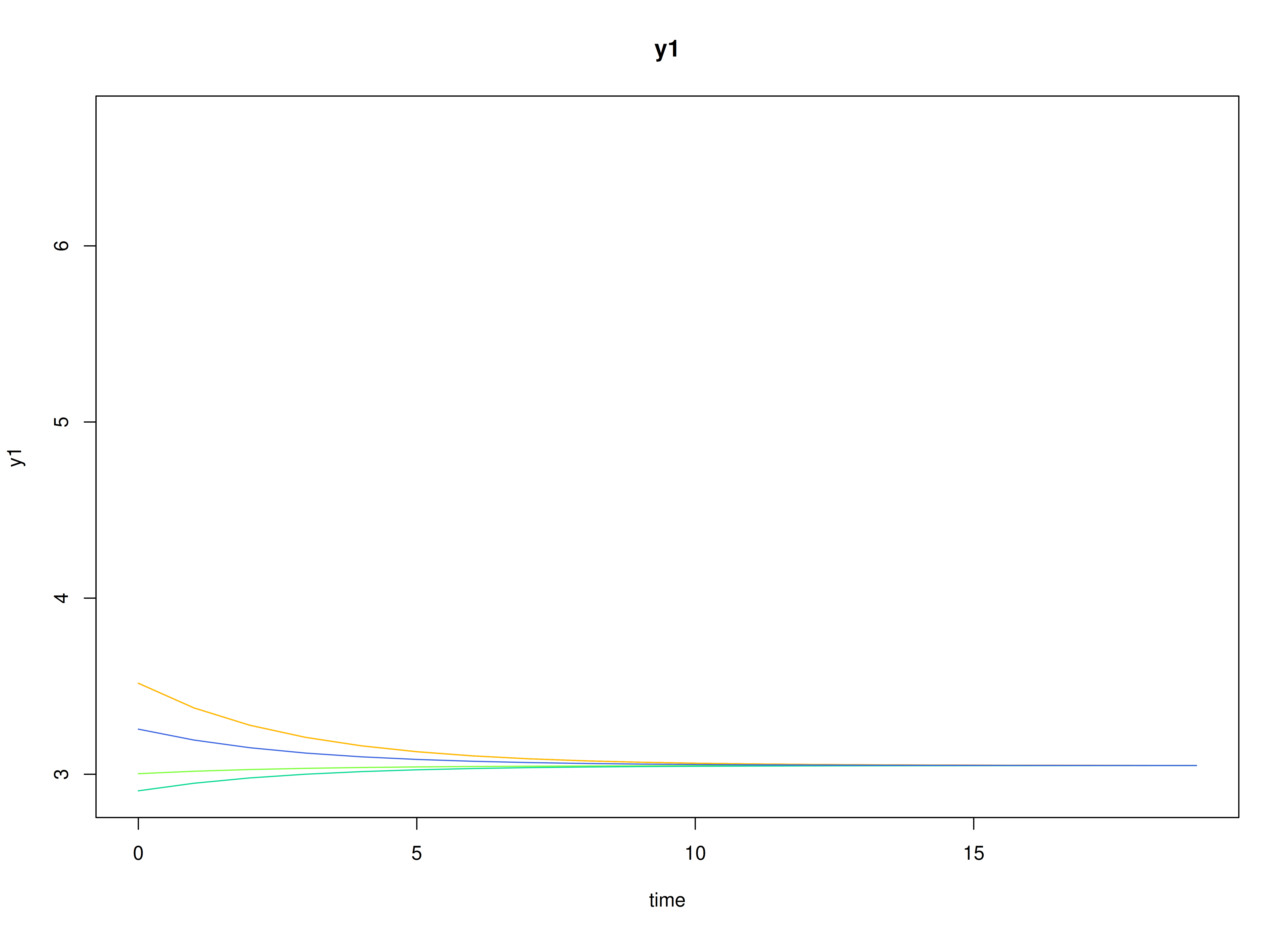

Visualizing the Dynamics Without Process Noise (n = 5 with Different Initial Condition)

Using the SimSSMVARFixed Function from the simStateSpace Package to Simulate Data

library(simStateSpace)
sim <- SimSSMVARFixed(
  n = n,
  time = time,
  mu0 = mu0,
  sigma0_l = sigma0_l,
  alpha = alpha,
  beta = beta,
  psi_l = psi_l
)
data <- as.data.frame(sim)
head(data)
#>   id time       y1       y2       y3
#> 1  1    0 3.375463 5.964917 3.883475
#> 2  1    1 3.136727 5.909374 3.866987
#> 3  1    2 3.215198 6.462812 3.995227
#> 4  1    3 3.427307 6.408953 4.408847
#> 5  1    4 3.108728 6.717274 5.303110
#> 6  1    5 3.885159 7.141896 5.024148
summary(data)
#>        id              time             y1              y2       
#>  Min.   :  1.00   Min.   :  0.0   Min.   :1.169   Min.   :3.552  
#>  1st Qu.: 25.75   1st Qu.:249.8   1st Qu.:2.755   1st Qu.:5.767  
#>  Median : 50.50   Median :499.5   Median :3.054   Median :6.160  
#>  Mean   : 50.50   Mean   :499.5   Mean   :3.055   Mean   :6.163  
#>  3rd Qu.: 75.25   3rd Qu.:749.2   3rd Qu.:3.356   3rd Qu.:6.558  
#>  Max.   :100.00   Max.   :999.0   Max.   :5.029   Max.   :8.619  
#>        y3       
#>  Min.   :2.460  
#>  1st Qu.:4.544  
#>  Median :4.893  
#>  Mean   :4.895  
#>  3rd Qu.:5.245  
#>  Max.   :7.672
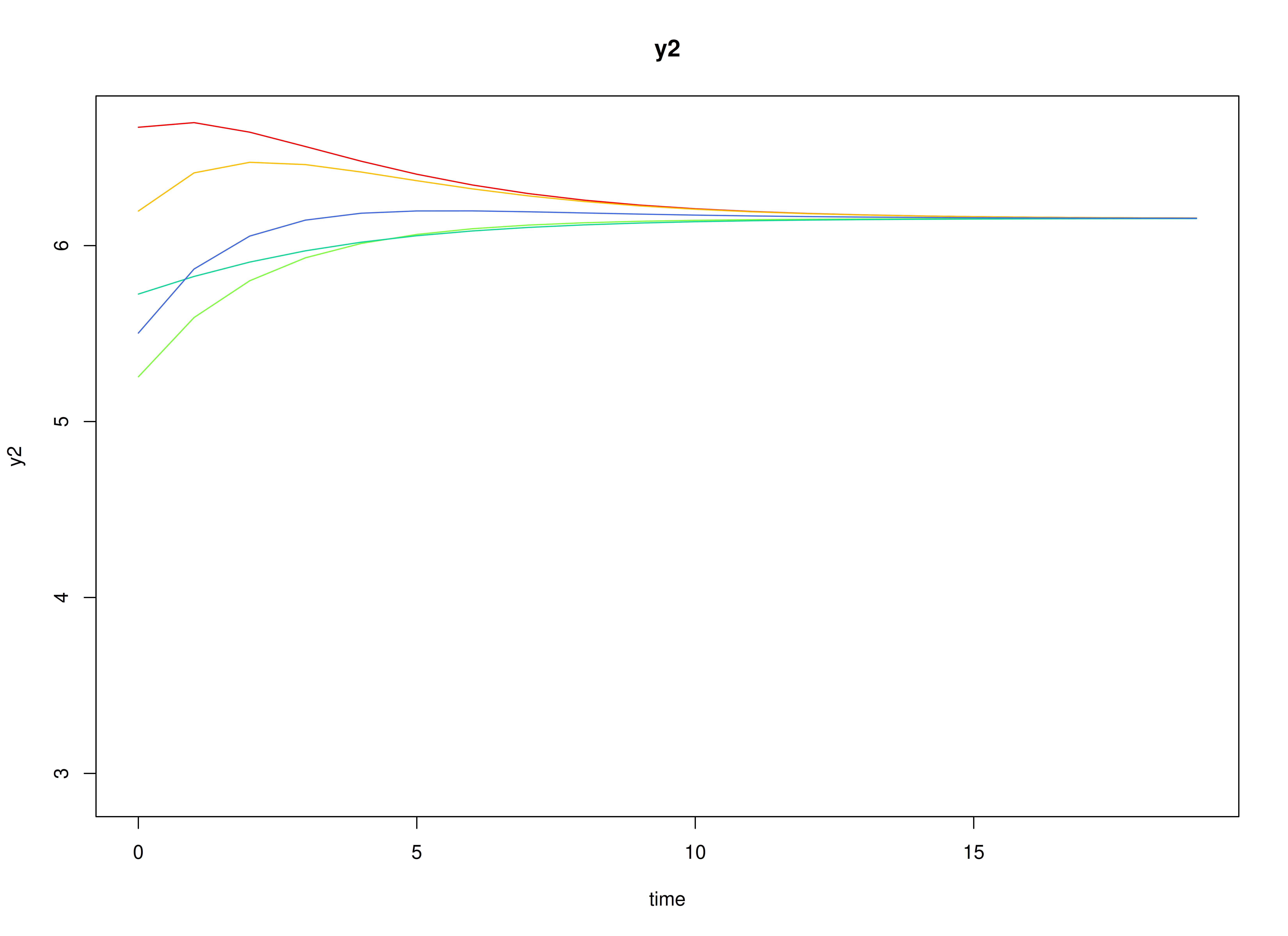
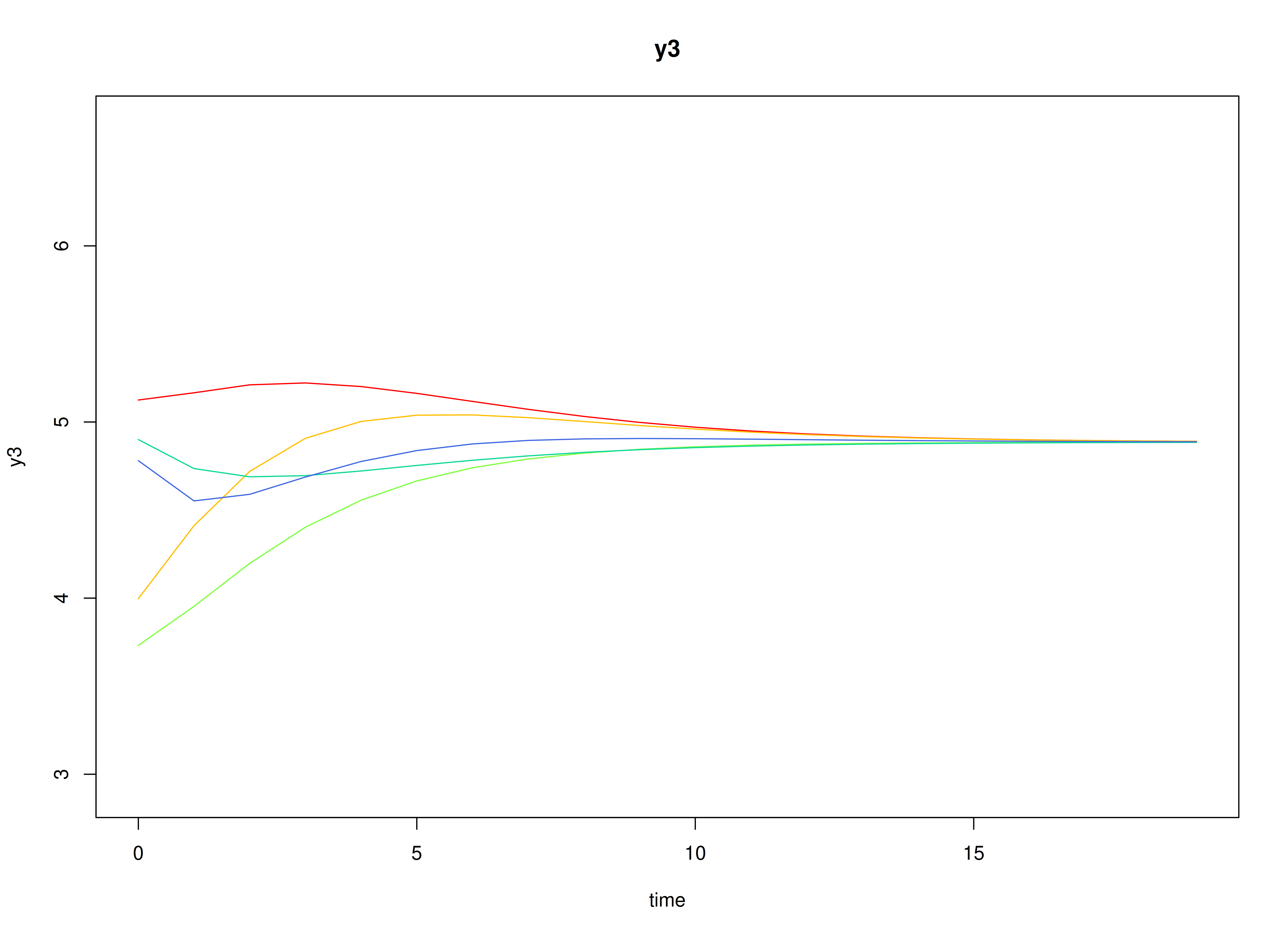
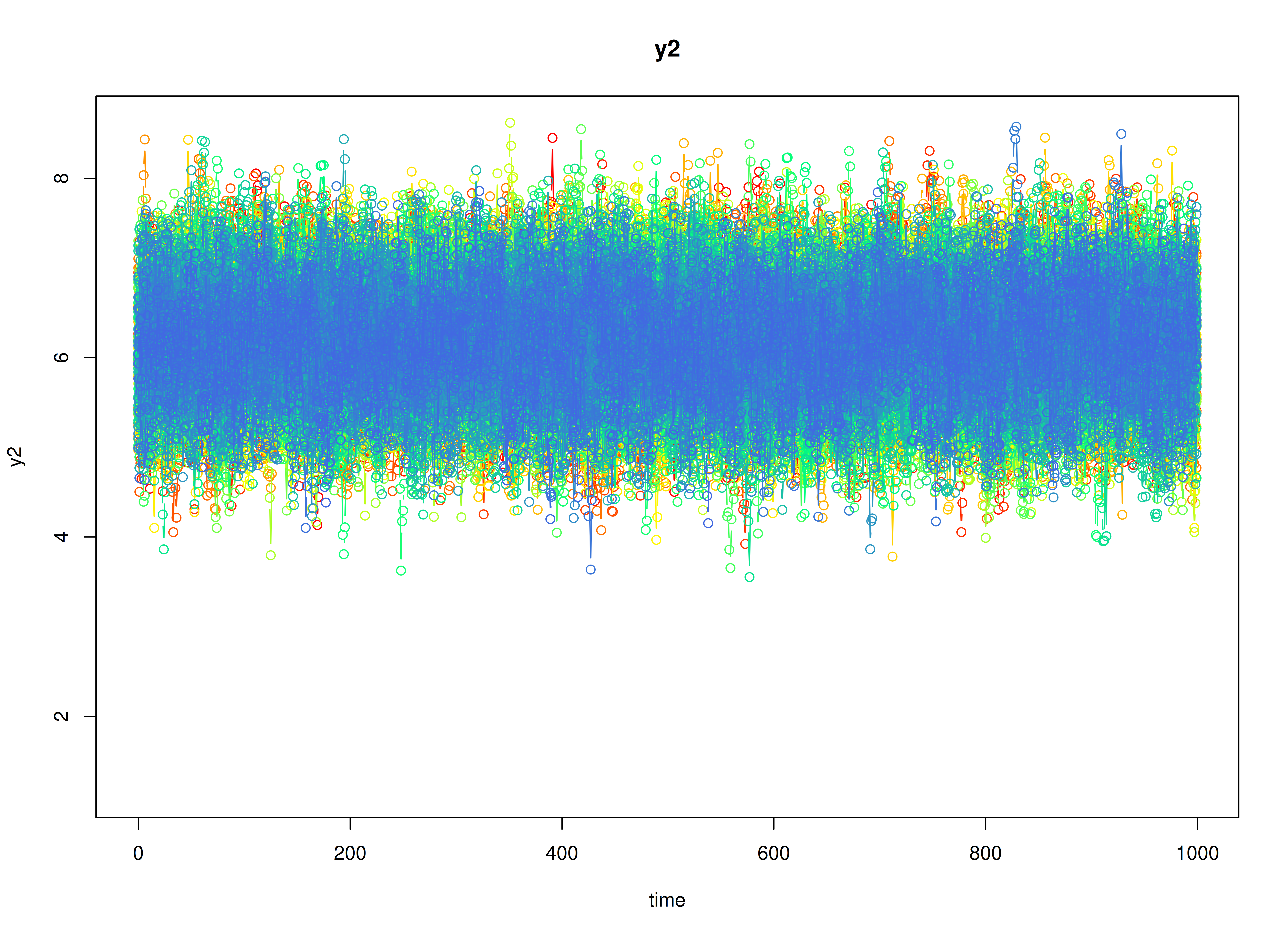
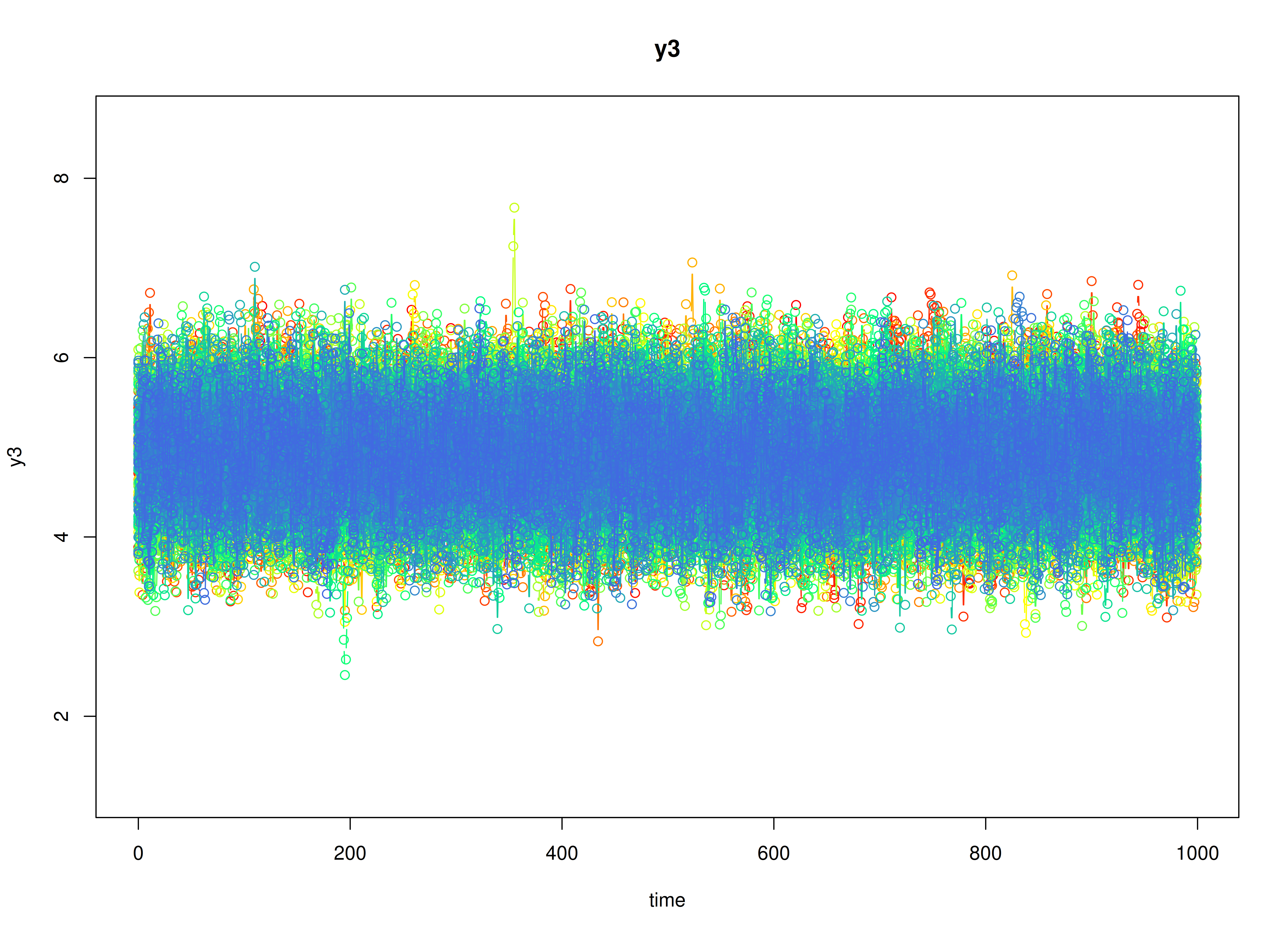
plot(sim)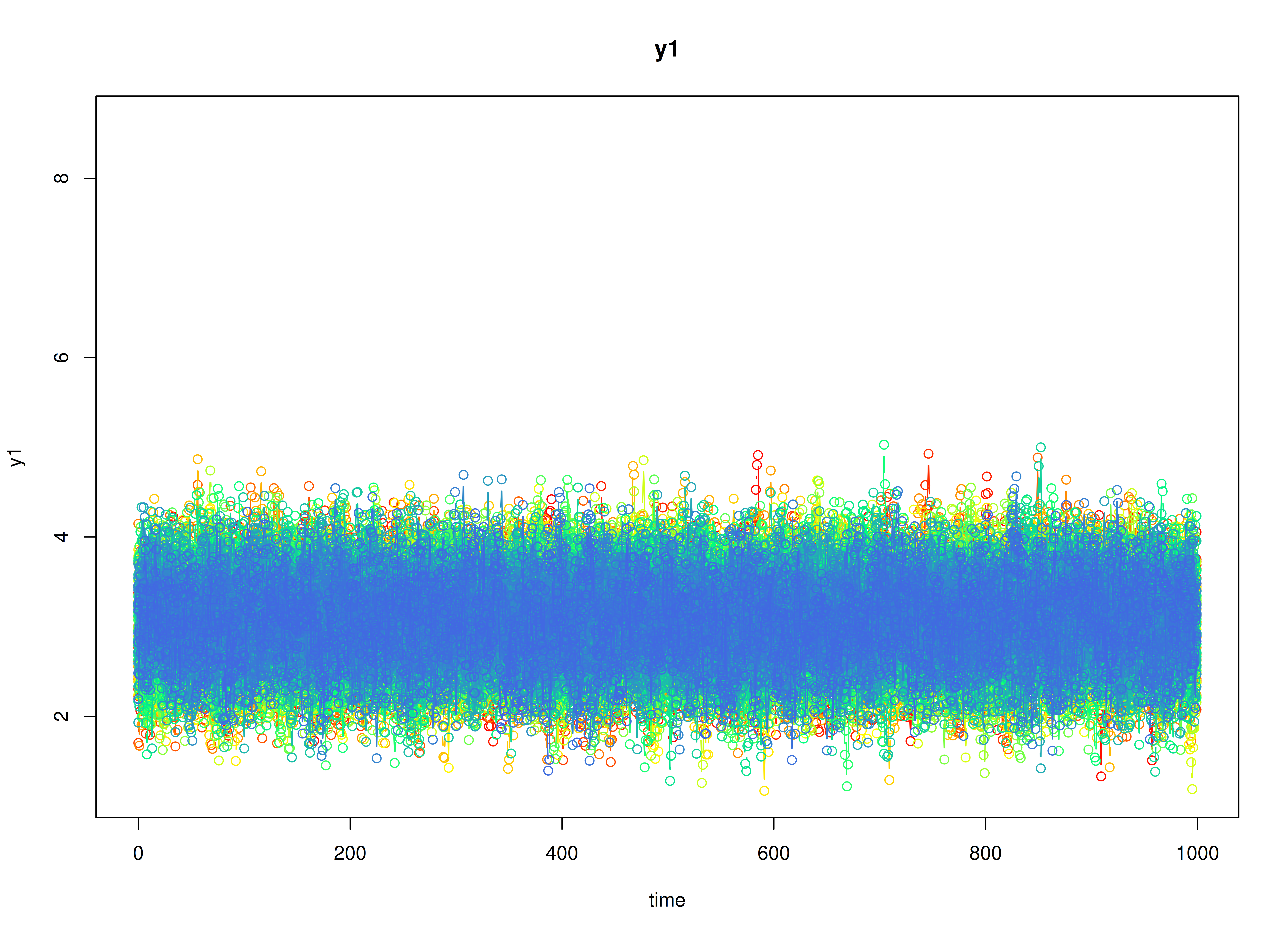

Model Fitting

library(OpenMx)
library(fitVARMxID)

The FitVARMxID function fits a DT-VAR model on each individual $i$.

Note: Consider using the argument ncores to use multiple cores for parallel processing.

fit <- FitVARMxID(
  data = data,
  observed = c("y1", "y2", "y3"),
  id = "id",
  center = TRUE,
  ncores = parallel::detectCores()
)

Parameter estimates

summary(
  fit,
  means = TRUE,
  ncores = parallel::detectCores()
)
#> Call:
#> FitVARMxID(data = data, observed = c("y1", "y2", "y3"), id = "id", 
#>     center = TRUE, ncores = parallel::detectCores())
#> 
#> Convergence:
#> 100.0%
#> 
#> Means of the estimated paramaters per individual.
#>   mu[1,1]   mu[2,1]   mu[3,1] beta[1,1] beta[2,1] beta[3,1] beta[1,2] beta[2,2] 
#>    3.0548    6.1622    4.8943    0.7001    0.4990   -0.0991   -0.0022    0.5998 
#> beta[3,2] beta[1,3] beta[2,3] beta[3,3]  psi[1,1]  psi[2,1]  psi[3,1]  psi[2,2] 
#>    0.4038   -0.0051   -0.0022    0.4982    0.0997    0.0004   -0.0003    0.0990 
#>  psi[3,2]  psi[3,3] 
#>    0.0005    0.0994

References

Hunter, M. D. (2017). State space modeling in an open source, modular, structural equation modeling environment. Structural Equation Modeling: A Multidisciplinary Journal, 25(2), 307–324. https://doi.org/10.1080/10705511.2017.1369354

Neale, M. C., Hunter, M. D., Pritikin, J. N., Zahery, M., Brick, T. R., Kirkpatrick, R. M., Estabrook, R., Bates, T. C., Maes, H. H., & Boker, S. M. (2015). OpenMx 2.0: Extended structural equation and statistical modeling. Psychometrika, 81(2), 535–549. https://doi.org/10.1007/s11336-014-9435-8

R Core Team. (2025). R: A language and environment for statistical computing. R Foundation for Statistical Computing. https://www.R-project.org/