Continuous-Time Vector Autoregressive Model (center = TRUE)

Ivan Jacob Agaloos Pesigan

2026-02-22

Model

The measurement model is given by $$\begin{equation} \mathbf{y}_{i, t} = \boldsymbol{\eta}_{i, t} \end{equation}$$ where $\mathbf{y}_{i, t}$, and $\boldsymbol{\eta}_{i, t}$ are random variables.

The dynamic structure is given by $$\begin{equation} \mathrm{d} \boldsymbol{\eta}_{i, t} = \boldsymbol{\beta}_{i} \left( \boldsymbol{\eta}_{i, t - 1} - \boldsymbol{\mu}_{i} \right) \mathrm{d} t + \boldsymbol{\Psi}_{i}^{\frac{1}{2}} \mathrm{d} \mathbf{W}_{i, t} \end{equation}$$ where $\mathrm{d}\boldsymbol{W}$ is a Wiener process or Brownian motion, which represents random fluctuations, $\boldsymbol{\eta}_{i, t}$, and $\boldsymbol{\eta}_{i, t - 1}$ are random variables, and $\boldsymbol{\mu}$, $\boldsymbol{\beta}$, and $\boldsymbol{\Psi}$ are model parameters. Here, $\boldsymbol{\eta}_{i, t}$ is a vector of latent variables at time $t$ and individual $i$, and $\boldsymbol{\eta}_{i, t - 1}$ represents a vector of latent variables at time $t - 1$ and individual $i$. $\boldsymbol{\mu}$ denotes a vector of set-points, $\boldsymbol{\beta}$ a matrix of auto and cross effect coefficients, and $\boldsymbol{\Psi}$ the covariance matrix of the random fluctuations.

Data Generation

Notation

Let $t = 1000$ be the number of time points and $n = 100$ be the number of individuals.

Let the initial condition $\boldsymbol{\eta}_{0}$ be given by

$$\begin{equation} \boldsymbol{\eta}_{0} \sim \mathcal{N} \left( \boldsymbol{\mu}_{\boldsymbol{\eta} \mid 0}, \boldsymbol{\Sigma}_{\boldsymbol{\eta} \mid 0} \right) \end{equation}$$

$$\begin{equation} \boldsymbol{\mu}_{\boldsymbol{\eta} \mid 0} = \left( \begin{array}{c} 2.5648173 \\ 5.7043283 \\ 4.7496423 \\ \end{array} \right) \end{equation}$$

$$\begin{equation} \boldsymbol{\Sigma}_{\boldsymbol{\eta} \mid 0} = \left( \begin{array}{ccc} 0.1401837 & 0.1245498 & 0.0264402 \\ 0.1245498 & 0.2858063 & 0.1435024 \\ 0.0264402 & 0.1435024 & 0.2059558 \\ \end{array} \right) . \end{equation}$$

Let the set-point vector $\boldsymbol{\mu}$ be given by

$$\begin{equation} \boldsymbol{\mu} = \left( \begin{array}{c} 2.5648173 \\ 5.7043283 \\ 4.7496423 \\ \end{array} \right) . \end{equation}$$

Let the transition matrix $\boldsymbol{\Phi}$ be given by

$$\begin{equation} \boldsymbol{\Phi} = \left( \begin{array}{ccc} -0.3566749 & 0 & 0 \\ 0.7707534 & -0.5108256 & 0 \\ -0.4499449 & 0.7292862 & -0.6931472 \\ \end{array} \right) . \end{equation}$$

Let the dynamic process noise $\boldsymbol{\Psi}$ be given by

$$\begin{equation} \boldsymbol{\Psi} = \left( \begin{array}{ccc} 0.1 & 0 & 0 \\ 0 & 0.1 & 0 \\ 0 & 0 & 0.1 \\ \end{array} \right) . \end{equation}$$

R Function Arguments

n
#> [1] 100
time
#> [1] 1000
mu0
#> [1] 2.564817 5.704328 4.749642
sigma0
#>            [,1]      [,2]       [,3]
#> [1,] 0.14018366 0.1245498 0.02644023
#> [2,] 0.12454982 0.2858063 0.14350238
#> [3,] 0.02644023 0.1435024 0.20595577
sigma0_l # sigma0_l <- t(chol(sigma0))
#>            [,1]      [,2]      [,3]
#> [1,] 0.37441109 0.0000000 0.0000000
#> [2,] 0.33265526 0.4185054 0.0000000
#> [3,] 0.07061819 0.2867606 0.3445827
alpha
#> [1] 0.9148060 0.9370754 0.2861395
beta
#>            [,1]       [,2]       [,3]
#> [1,] -0.3566749  0.0000000  0.0000000
#> [2,]  0.7707534 -0.5108256  0.0000000
#> [3,] -0.4499449  0.7292862 -0.6931472
psi
#>      [,1] [,2] [,3]
#> [1,]  0.1  0.0  0.0
#> [2,]  0.0  0.1  0.0
#> [3,]  0.0  0.0  0.1
psi_l # psi_l <- t(chol(psi))
#>           [,1]      [,2]      [,3]
#> [1,] 0.3162278 0.0000000 0.0000000
#> [2,] 0.0000000 0.3162278 0.0000000
#> [3,] 0.0000000 0.0000000 0.3162278
# set-point
mu
#> [1] 2.564817 5.704328 4.749642
nu
#> [1] 0 0 0
lambda
#>      [,1] [,2] [,3]
#> [1,]    1    0    0
#> [2,]    0    1    0
#> [3,]    0    0    1
theta
#>      [,1] [,2] [,3]
#> [1,]    0    0    0
#> [2,]    0    0    0
#> [3,]    0    0    0

Visualizing the Dynamics Without Process Noise (n = 5 with Different Initial Condition)

Using the SimSSMLinSDEFixed Function from the simStateSpace Package to Simulate Data

Note: The SimSSMLinSDEFixed function uses a different set of parameter names. See help(SimSSMLinSDEFixed) for more details.

library(simStateSpace)
sim <- SimSSMLinSDEFixed(
  n = n,
  time = time,
  delta_t = 0.1,
  mu0 = mu0,
  sigma0_l = sigma0_l,
  iota = alpha,
  phi = beta,
  sigma_l = psi_l,
  nu = nu,
  lambda = lambda,
  theta_l = theta_l
)
data <- as.data.frame(sim)
head(data)
#>   id time       y1       y2       y3
#> 1  1  0.0 2.713440 6.616955 5.826304
#> 2  1  0.1 2.788586 6.625107 5.689081
#> 3  1  0.2 2.752473 6.722281 5.621800
#> 4  1  0.3 2.504163 6.706956 5.588982
#> 5  1  0.4 2.541571 6.800410 5.517594
#> 6  1  0.5 2.499550 6.830410 5.316913
summary(data)
#>        id              time             y1              y2       
#>  Min.   :  1.00   Min.   : 0.00   Min.   :1.197   Min.   :3.688  
#>  1st Qu.: 25.75   1st Qu.:24.98   1st Qu.:2.307   1st Qu.:5.342  
#>  Median : 50.50   Median :49.95   Median :2.561   Median :5.709  
#>  Mean   : 50.50   Mean   :49.95   Mean   :2.561   Mean   :5.709  
#>  3rd Qu.: 75.25   3rd Qu.:74.92   3rd Qu.:2.811   3rd Qu.:6.067  
#>  Max.   :100.00   Max.   :99.90   Max.   :4.172   Max.   :8.164  
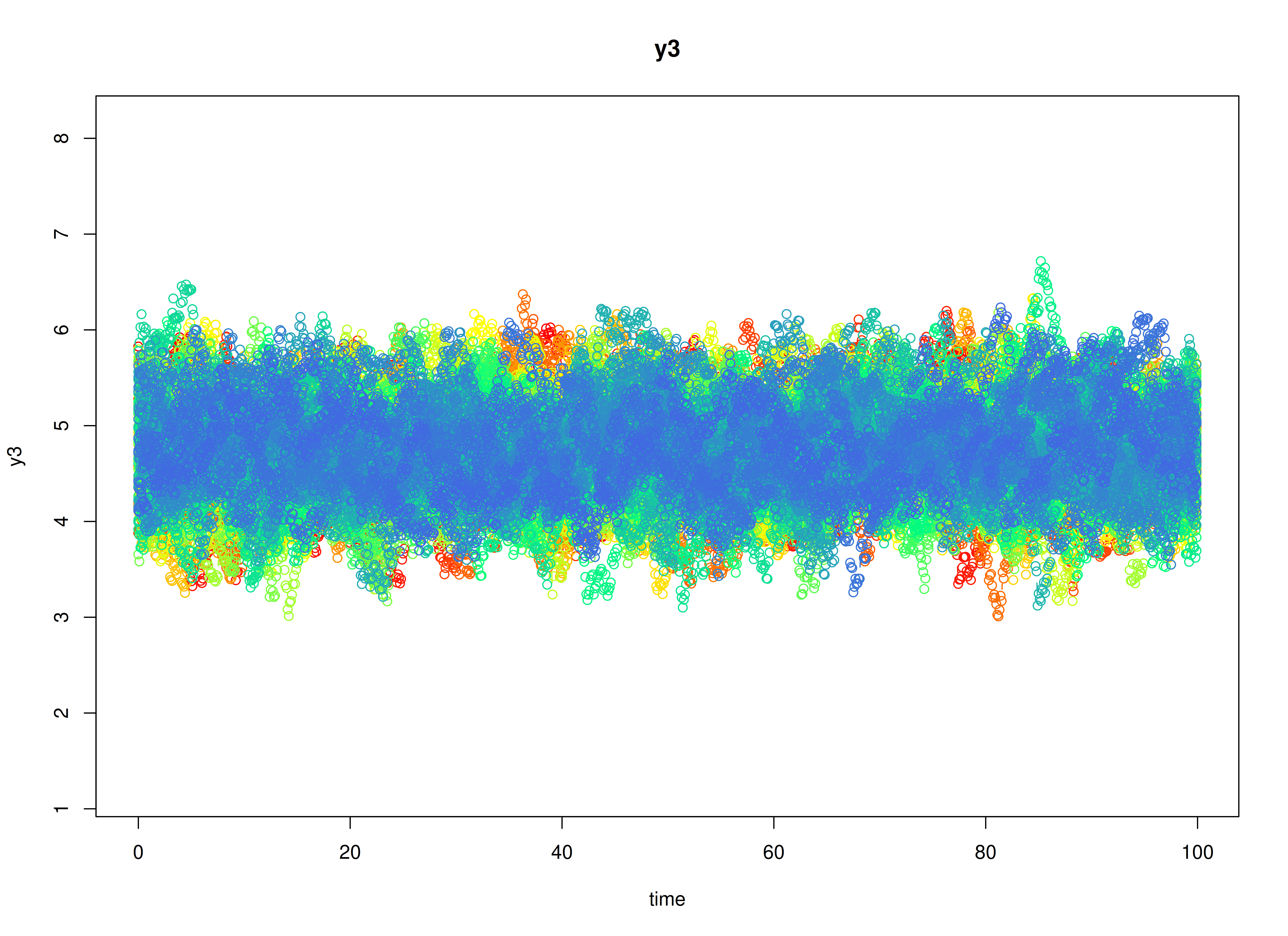
#>        y3       
#>  Min.   :3.009  
#>  1st Qu.:4.455  
#>  Median :4.751  
#>  Mean   :4.755  
#>  3rd Qu.:5.054  
#>  Max.   :6.718
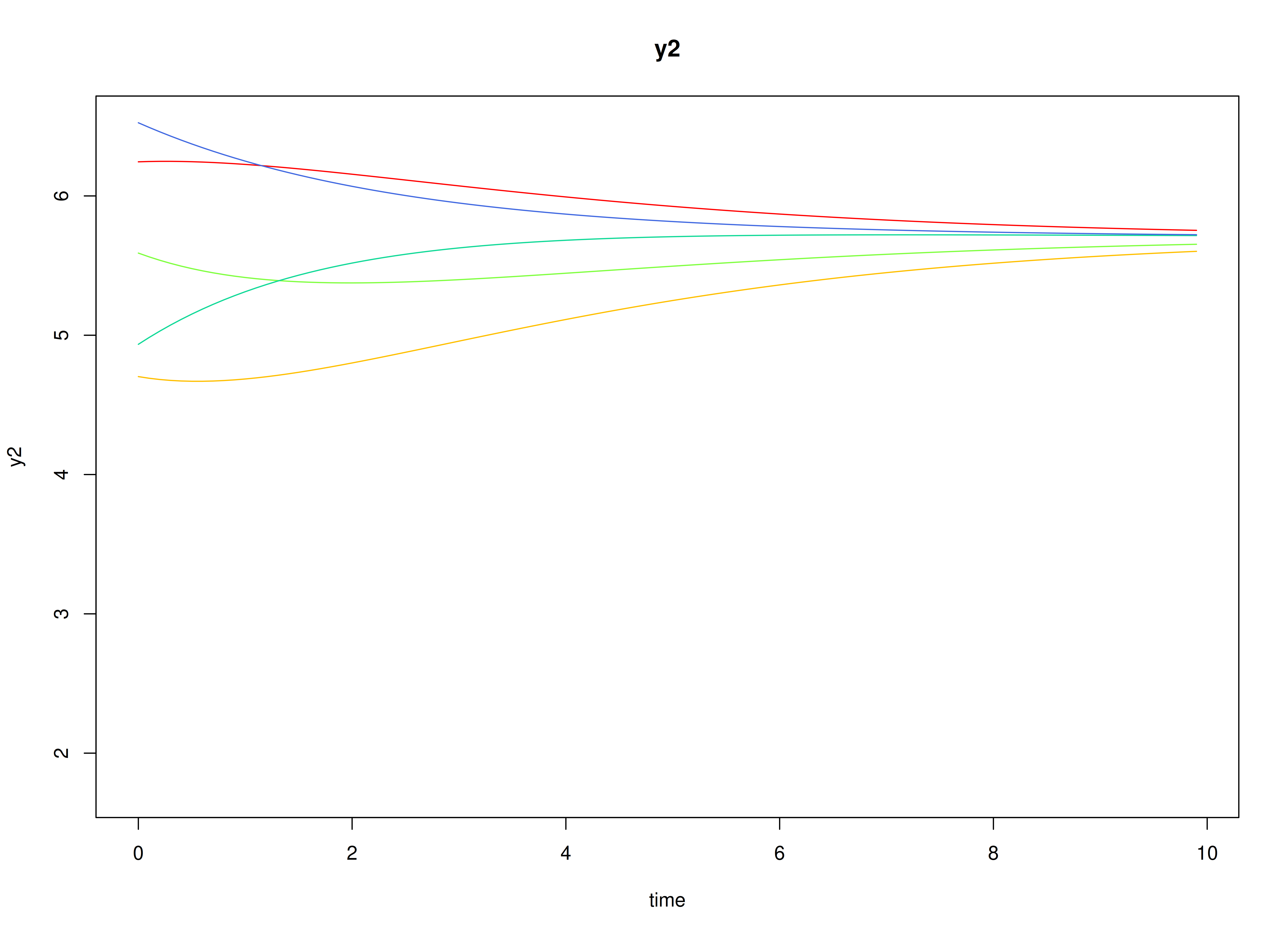
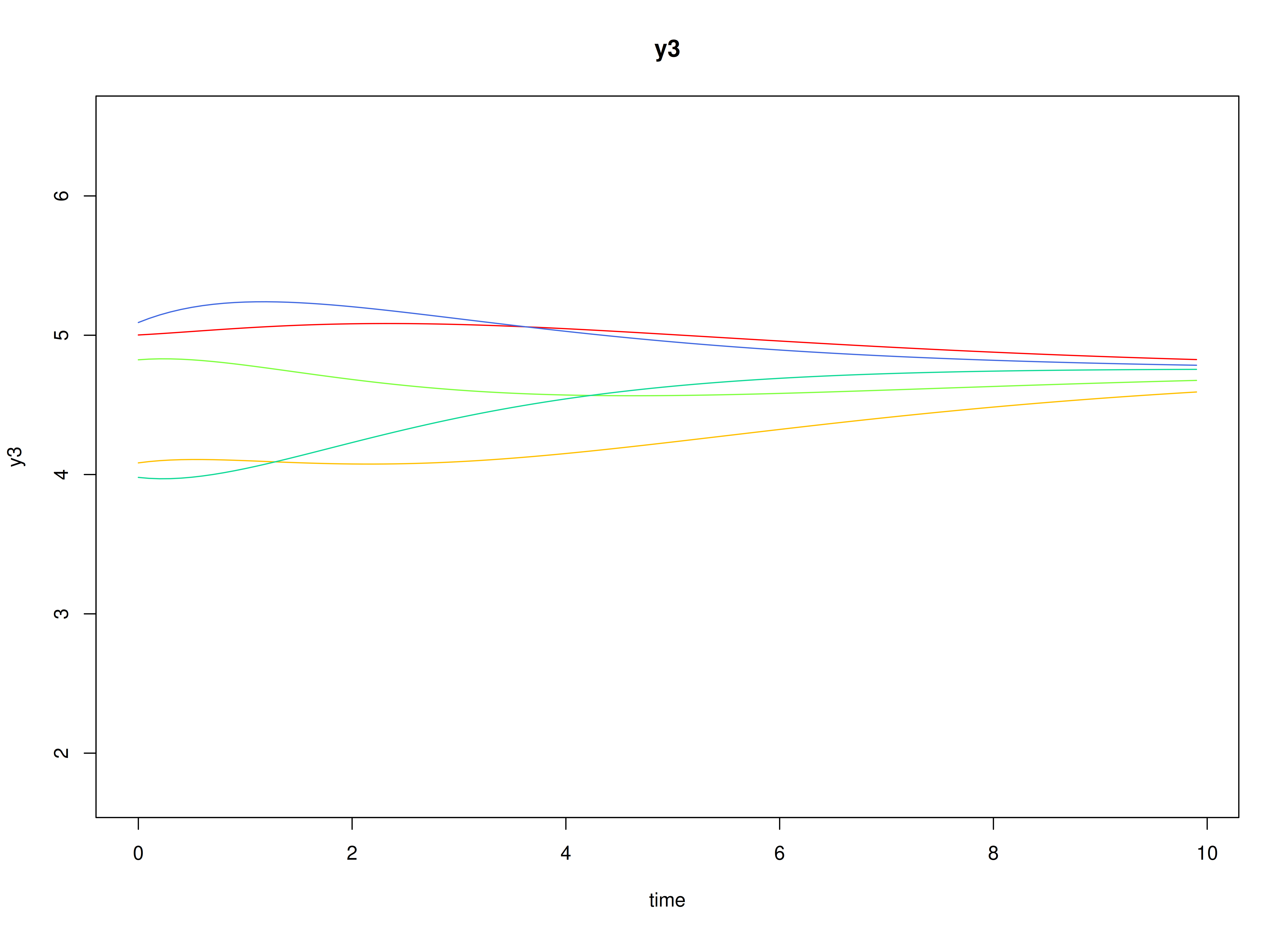
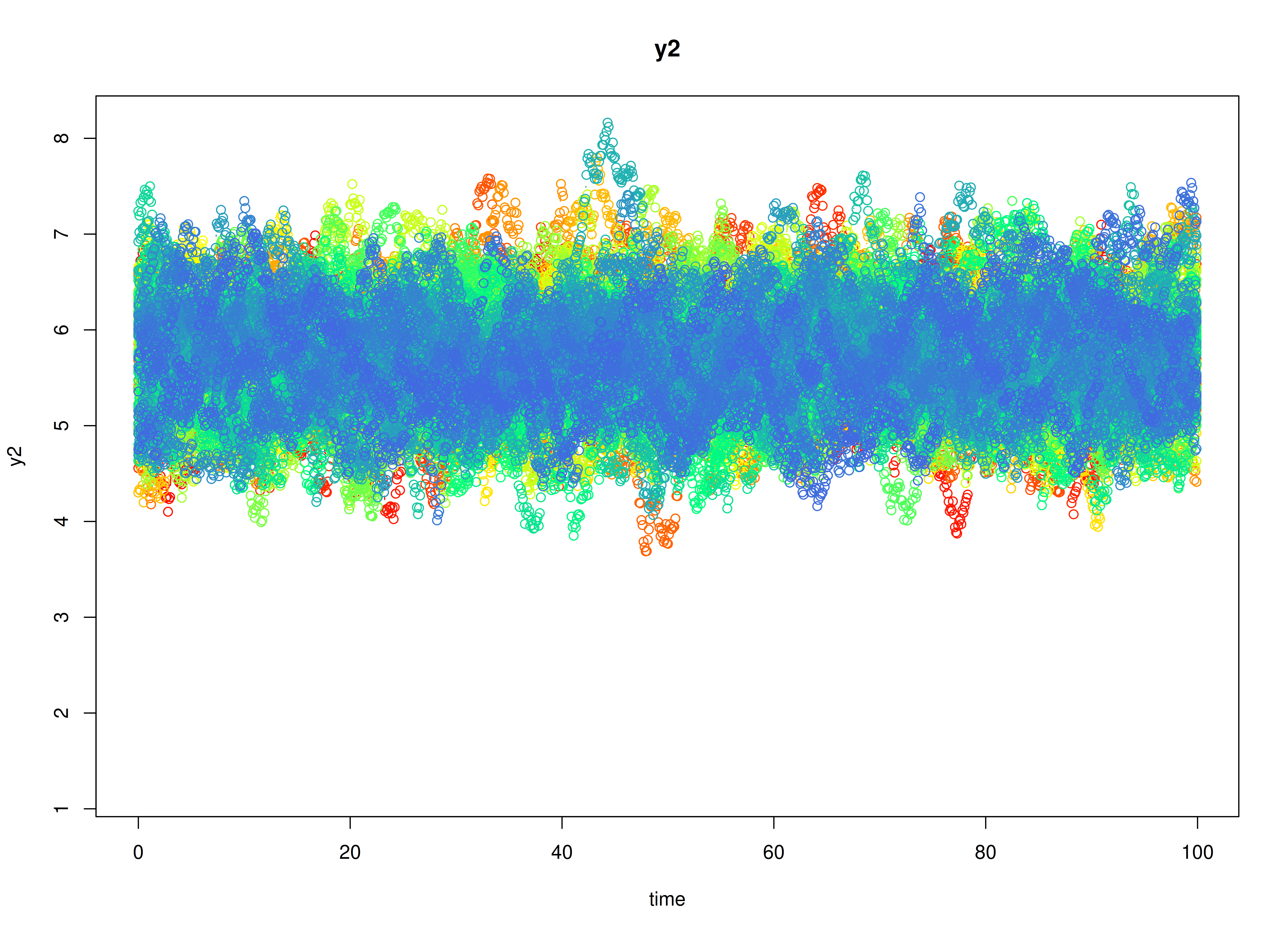
plot(sim)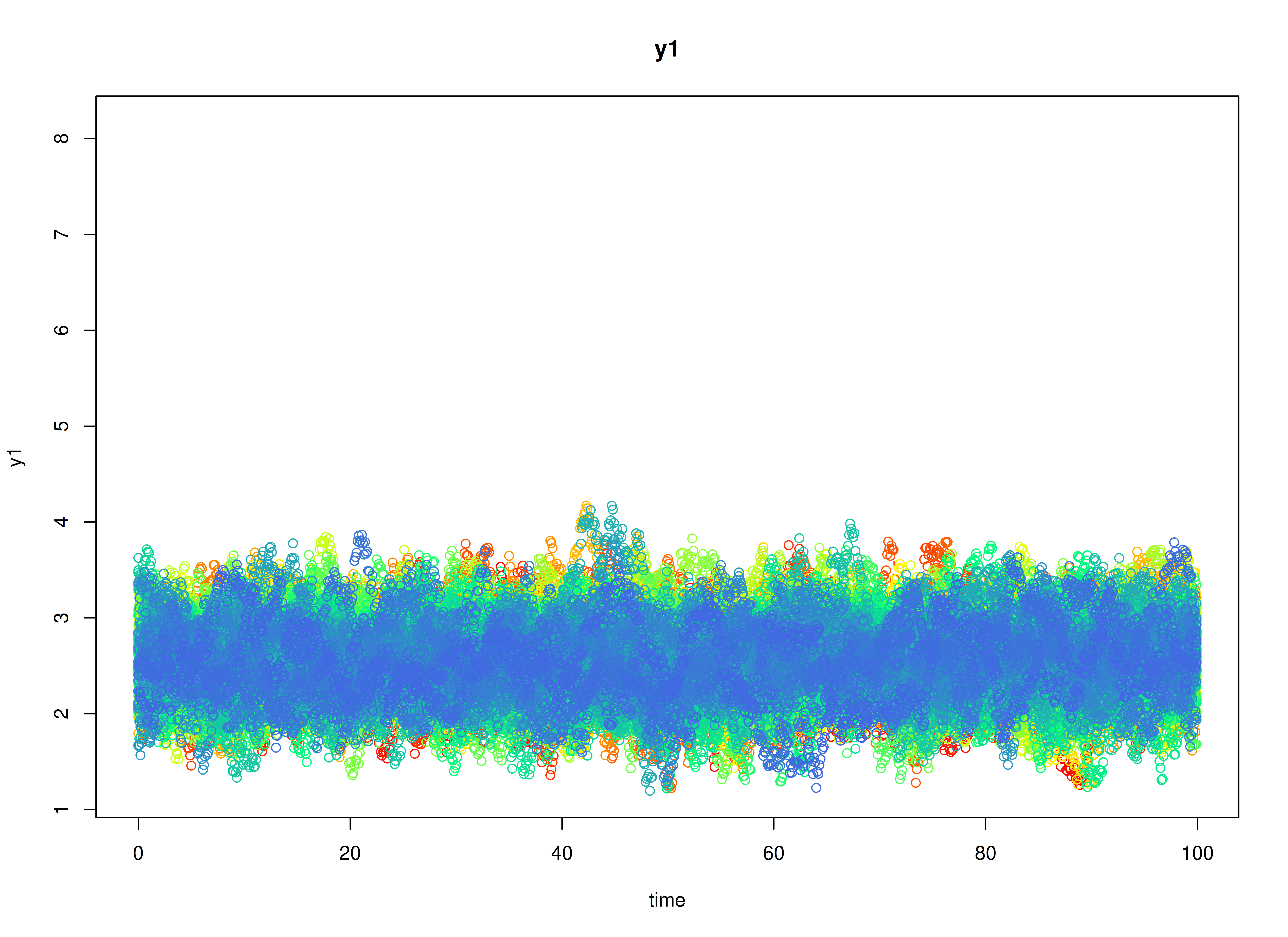

Model Fitting

library(OpenMx)
library(fitVARMxID)

The FitVARMxID function fits a CT-VAR model on each individual $i$.

Note: Consider using the argument ncores to use multiple cores for parallel processing.

fit <- FitVARMxID(
  data = data,
  observed = c("y1", "y2", "y3"),
  id = "id",
  ct = TRUE,
  time = "time",
  center = TRUE,
  ncores = parallel::detectCores()
)

Parameter estimates

summary(
  fit,
  means = TRUE,
  ncores = parallel::detectCores()
)
#> Call:
#> FitVARMxID(data = data, observed = c("y1", "y2", "y3"), id = "id", 
#>     time = "time", ct = TRUE, center = TRUE, ncores = parallel::detectCores())
#> 
#> Convergence:
#> 100.0%
#> 
#> Means of the estimated paramaters per individual.
#>   mu[1,1]   mu[2,1]   mu[3,1] beta[1,1] beta[2,1] beta[3,1] beta[1,2] beta[2,2] 
#>    2.5623    5.7117    4.7566   -0.4118    0.7893   -0.4533   -0.0064   -0.5344 
#> beta[3,2] beta[1,3] beta[2,3] beta[3,3]  psi[1,1]  psi[2,1]  psi[3,1]  psi[2,2] 
#>    0.7514   -0.0148   -0.0200   -0.7402    0.1007    0.0003   -0.0002    0.0993 
#>  psi[3,2]  psi[3,3] 
#>    0.0003    0.1003

References

Hunter, M. D. (2017). State space modeling in an open source, modular, structural equation modeling environment. Structural Equation Modeling: A Multidisciplinary Journal, 25(2), 307–324. https://doi.org/10.1080/10705511.2017.1369354

Neale, M. C., Hunter, M. D., Pritikin, J. N., Zahery, M., Brick, T. R., Kirkpatrick, R. M., Estabrook, R., Bates, T. C., Maes, H. H., & Boker, S. M. (2015). OpenMx 2.0: Extended structural equation and statistical modeling. Psychometrika, 81(2), 535–549. https://doi.org/10.1007/s11336-014-9435-8

R Core Team. (2025). R: A language and environment for statistical computing. R Foundation for Statistical Computing. https://www.R-project.org/