Fit the Discrete-Time Vector Autoregressive Model

Model

The measurement model is given by $\begin{equation} \mathbf{y}_{i, t} = \boldsymbol{\Lambda} \boldsymbol{\eta}_{i, t} + \boldsymbol{\varepsilon}_{i, t}, \quad \mathrm{with} \quad \boldsymbol{\varepsilon}_{i, t} \sim \mathcal{N} \left( \mathbf{0}, \boldsymbol{\Theta} \right) \end{equation}$ where $\mathbf{y}_{i, t}$ , $\boldsymbol{\eta}_{i, t}$ , and $\boldsymbol{\varepsilon}_{i, t}$ are random variables and $\boldsymbol{\Lambda}$ , and $\boldsymbol{\Theta}$ are model parameters. $\mathbf{y}_{i, t}$ represents a vector of observed random variables, $\boldsymbol{\eta}_{i, t}$ a vector of latent random variables, and $\boldsymbol{\varepsilon}_{i, t}$ a vector of random measurement errors, at time $t$ and individual $i$ . $\boldsymbol{\Lambda}$ denotes a matrix of factor loadings, and $\boldsymbol{\Theta}$ the covariance matrix of $\boldsymbol{\varepsilon}$ . In this model, $\boldsymbol{\Lambda}$ is an identity matrix and $\boldsymbol{\Theta}$ is a diagonal matrix.

The dynamic structure is given by $\begin{equation} \boldsymbol{\eta}_{i, t} = \boldsymbol{\alpha} + \boldsymbol{\beta} \boldsymbol{\eta}_{i, t - 1} + \boldsymbol{\zeta}_{i, t}, \quad \mathrm{with} \quad \boldsymbol{\zeta}_{i, t} \sim \mathcal{N} \left( \mathbf{0}, \boldsymbol{\Psi} \right) \end{equation}$ where $\boldsymbol{\eta}_{i, t}$ , $\boldsymbol{\eta}_{i, t - 1}$ , and $\boldsymbol{\zeta}_{i, t}$ are random variables, and $\boldsymbol{\alpha}$ , $\boldsymbol{\beta}$ , and $\boldsymbol{\Psi}$ are model parameters. Here, $\boldsymbol{\eta}_{i, t}$ is a vector of latent variables at time $t$ and individual $i$ , $\boldsymbol{\eta}_{i, t - 1}$ represents a vector of latent variables at time $t - 1$ and individual $i$ , and $\boldsymbol{\zeta}_{i, t}$ represents a vector of dynamic noise at time $t$ and individual $i$ . $\boldsymbol{\alpha}$ denotes a vector of intercepts, $\boldsymbol{\beta}$ a matrix of autoregression and cross regression coefficients, and $\boldsymbol{\Psi}$ the covariance matrix of $\boldsymbol{\zeta}_{i, t}$ . In this model, $\boldsymbol{\Psi}$ is a symmetric matrix.

Data Generation

The parameters used in this example were based on Bringmann et al. (2013).

Notation

Let $t = 1000$ be the number of time points and $n = 1000$ be the number of individuals.

Let the measurement model intecept vector $\boldsymbol{\nu}$ be given by

$\begin{equation} \boldsymbol{\nu} = \left( \begin{array}{c} 0 \\ 0 \\ \end{array} \right) . \end{equation}$

Let the factor loadings matrix $\boldsymbol{\Lambda}$ be given by

$\begin{equation} \boldsymbol{\Lambda} = \left( \begin{array}{cc} 1 & 0 \\ 0 & 1 \\ \end{array} \right) . \end{equation}$

Let the measurement error covariance matrix $\boldsymbol{\Theta}$ be given by

$\begin{equation} \boldsymbol{\Theta} = \left( \begin{array}{cc} 0.2 & 0 \\ 0 & 0.2 \\ \end{array} \right) . \end{equation}$

Let the initial condition $\boldsymbol{\eta}_{0}$ be given by

$\begin{equation} \boldsymbol{\eta}_{0} \sim \mathcal{N} \left( \boldsymbol{\mu}_{\boldsymbol{\eta} \mid 0}, \boldsymbol{\Sigma}_{\boldsymbol{\eta} \mid 0} \right) \end{equation}$

$\begin{equation} \boldsymbol{\mu}_{\boldsymbol{\eta} \mid 0} = \left( \begin{array}{c} 3.8143546 \\ 2.5763481 \\ \end{array} \right) \end{equation}$

$\begin{equation} \boldsymbol{\Sigma}_{\boldsymbol{\eta} \mid 0} = \left( \begin{array}{cc} 1.3978842 & 0.5782369 \\ 0.5782369 & 1.6636513 \\ \end{array} \right) . \end{equation}$

Let the transition matrix $\boldsymbol{\beta}$ be given by

$\begin{equation} \left( \begin{array}{cc} 0.28 & -0.048 \\ -0.035 & 0.26 \\ \end{array} \right) . \end{equation}$

Let the dynamic process noise $\boldsymbol{\Psi}$ be given by

$\begin{equation} \boldsymbol{\Psi} = \left( \begin{array}{cc} 1.3 & 0.5696315 \\ 0.5696315 & 1.56 \\ \end{array} \right) . \end{equation}$

R Function Arguments

n
#> [1] 1000
time
#> [1] 1000
mu0
#> [1] 3.814355 2.576348
sigma0
#>           [,1]      [,2]
#> [1,] 1.3978842 0.5782369
#> [2,] 0.5782369 1.6636513
sigma0_l # sigma0_l <- t(chol(sigma0))
#>           [,1]     [,2]
#> [1,] 1.1823215 0.000000
#> [2,] 0.4890691 1.193509
alpha
#> [1] 2.87 2.04
beta
#>        [,1]   [,2]
#> [1,]  0.280 -0.048
#> [2,] -0.035  0.260
psi
#>           [,1]      [,2]
#> [1,] 1.3000000 0.5696315
#> [2,] 0.5696315 1.5600000
psi_l # psi_l <- t(chol(psi))
#>           [,1]     [,2]
#> [1,] 1.1401754 0.000000
#> [2,] 0.4995998 1.144727
nu
#> [1] 0 0
lambda
#>      [,1] [,2]
#> [1,]    1    0
#> [2,]    0    1
theta
#>      [,1] [,2]
#> [1,]  0.2  0.0
#> [2,]  0.0  0.2
theta_l # theta_l <- t(chol(theta))
#>           [,1]      [,2]
#> [1,] 0.4472136 0.0000000
#> [2,] 0.0000000 0.4472136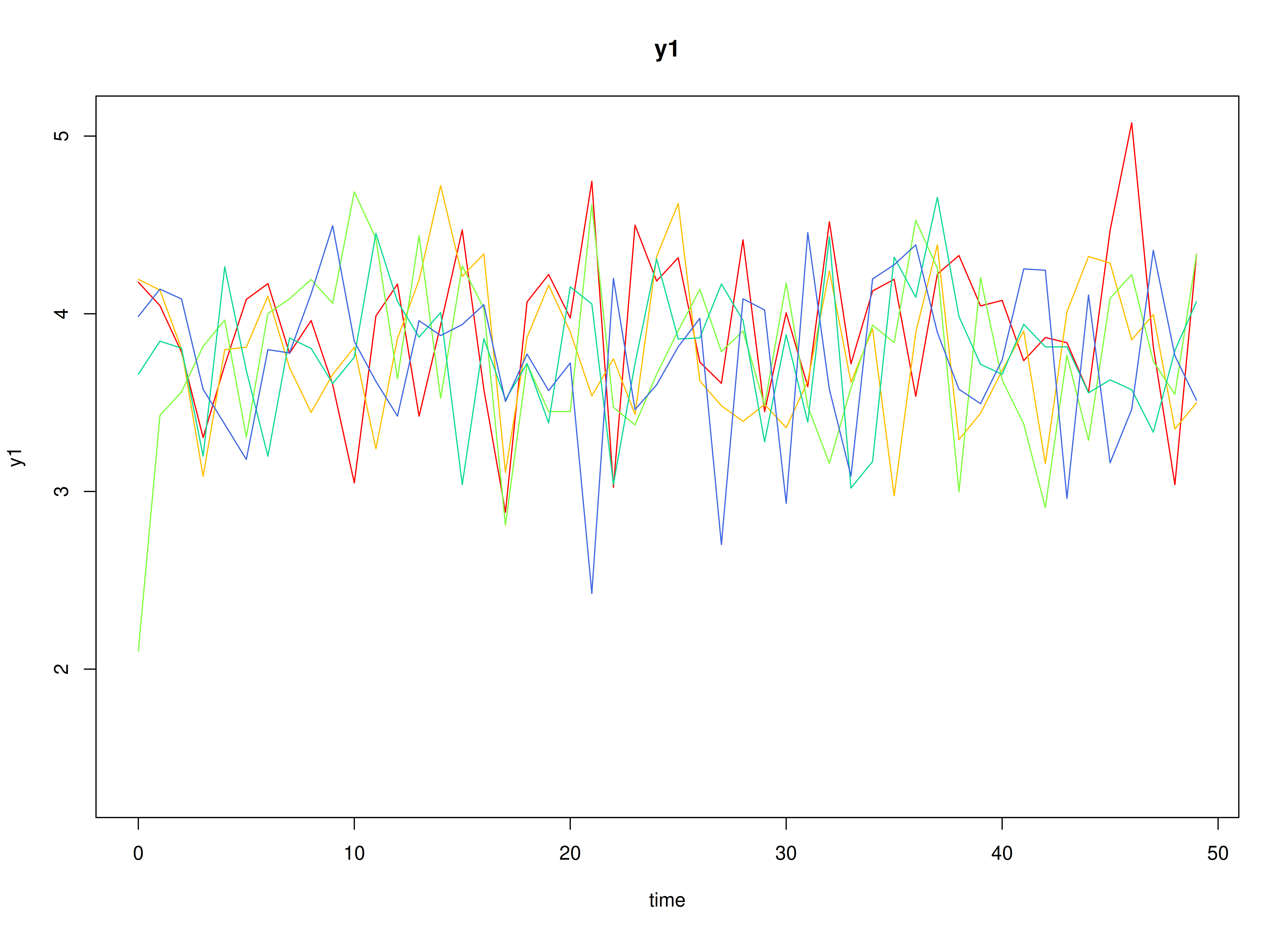

Visualizing the Dynamics Without Process Noise (n = 5 with Different Initial Condition)

Using the `SimSSMFixed` Function from the `simStateSpace` Package to Simulate Data

library(simStateSpace)
sim <- SimSSMFixed(
  n = n,
  time = time,
  mu0 = mu0,
  sigma0_l = sigma0_l,
  alpha = alpha,
  beta = beta,
  psi_l = psi_l,
  nu = nu,
  lambda = lambda,
  theta_l = theta_l
)
data <- as.data.frame(sim)
head(data)
#>   id time       y1        y2
#> 1  1    0 3.455114 1.9223092
#> 2  1    1 5.696312 0.6452660
#> 3  1    2 4.364664 1.4954592
#> 4  1    3 4.900281 2.6730811
#> 5  1    4 2.325515 0.2139305
#> 6  1    5 3.340405 1.9930331
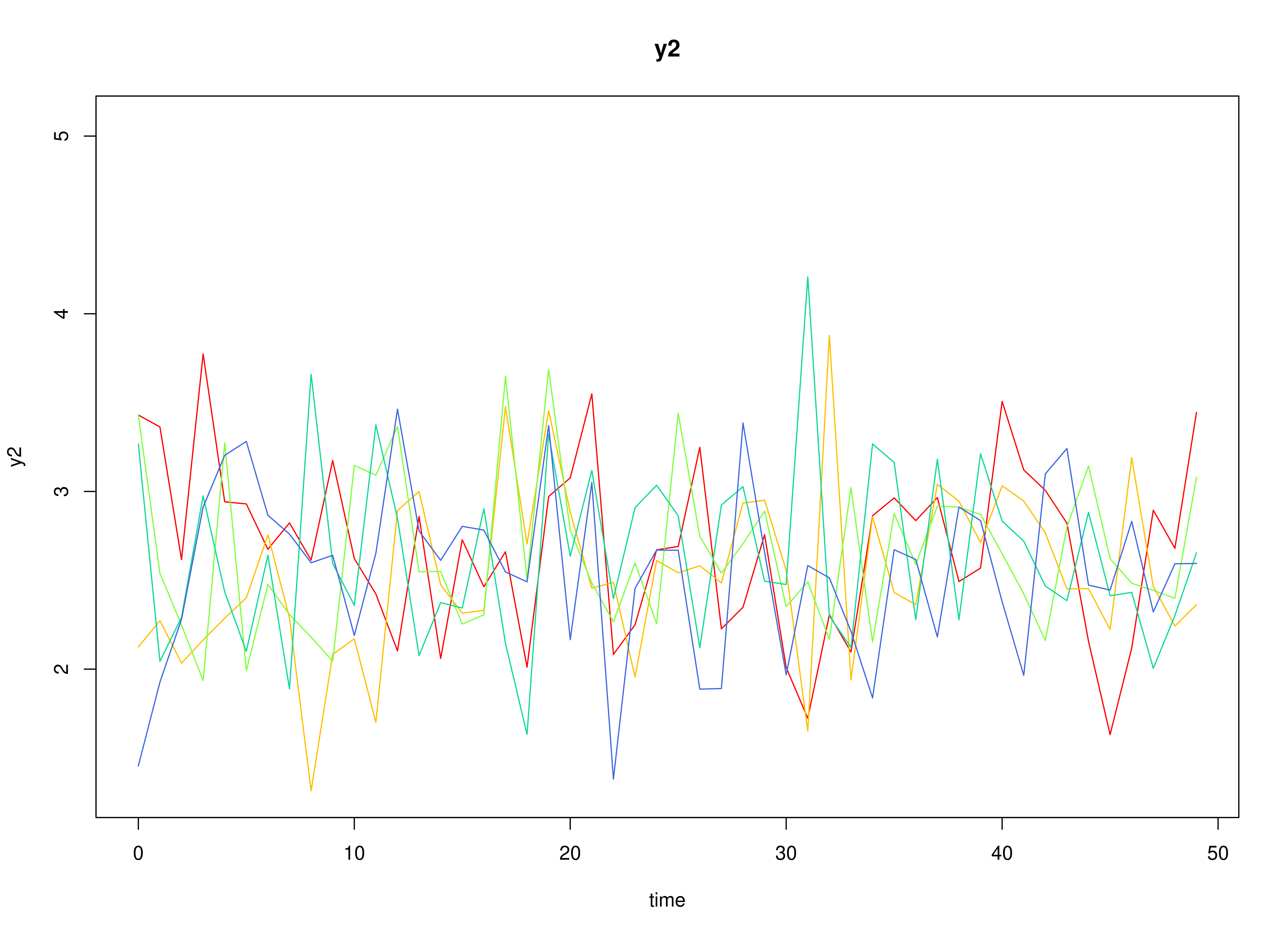
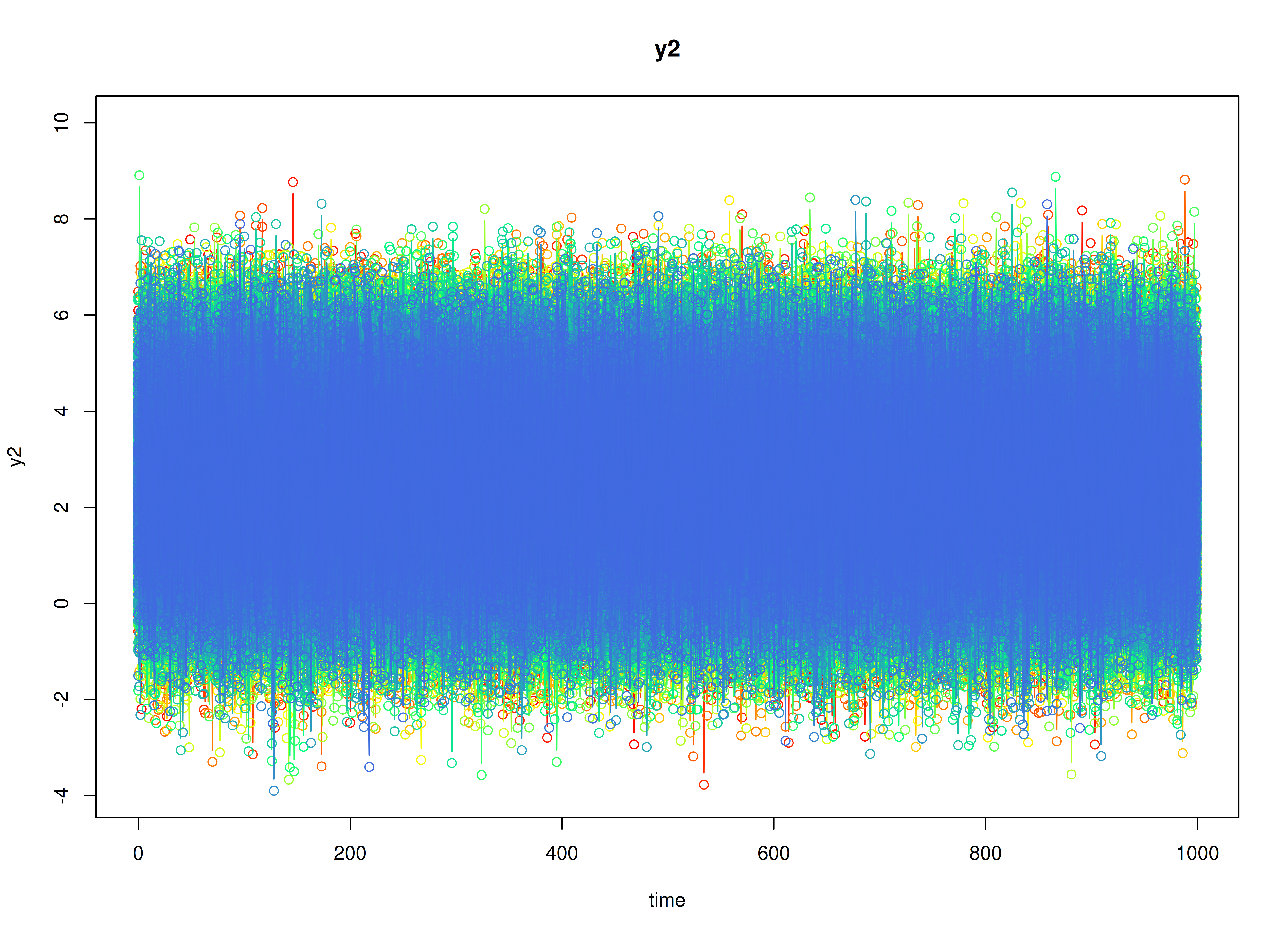
plot(sim)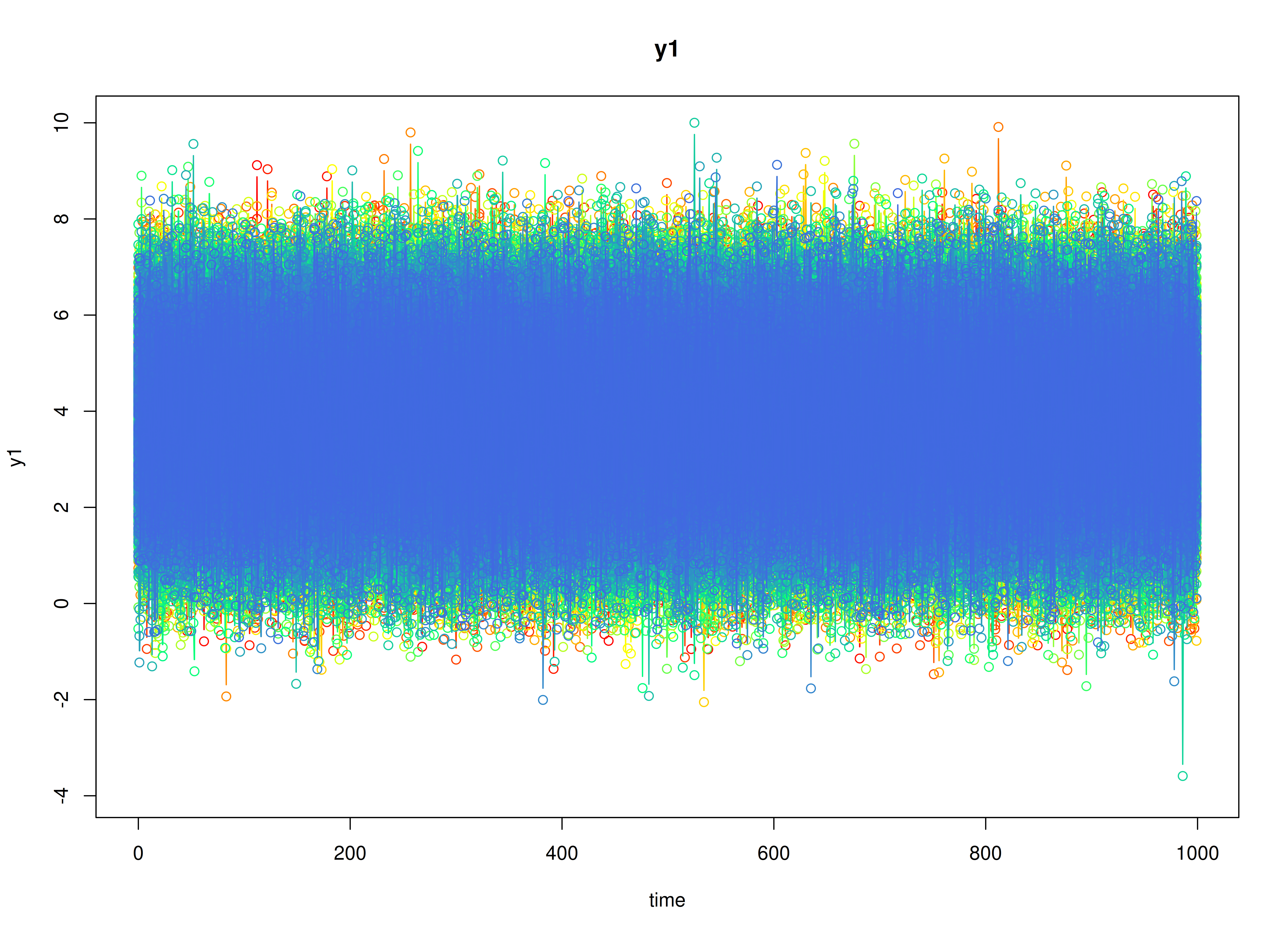

Model Fitting

The FitDTVARMx function fits a DT-VAR model assuming fixed parameters.

library(fitDTVARMx)
fit <- FitDTVARMx(
  data = data,
  observed = paste0("y", seq_len(k)),
  id = "id",
  ncores = parallel::detectCores()
)
#> Running DTVAR with 16 parameters
#> 
#> Beginning initial fit attempt
#> Running DTVAR with 16 parameters
#> 
#>  Fit attempt generated errors
#> 
#> Beginning fit attempt 1 of at maximum 1000 extra tries
#> Running DTVAR with 16 parameters
#> 
#>  Fit attempt generated errors
#> 
#> Beginning fit attempt 2 of at maximum 1000 extra tries
#> Running DTVAR with 16 parameters
#> 
#>  Fit attempt generated errors
#> 
#> Beginning fit attempt 3 of at maximum 1000 extra tries
#> Running DTVAR with 16 parameters
#> 
#>  Fit attempt generated errors
#> 
#> Beginning fit attempt 4 of at maximum 1000 extra tries
#> Running DTVAR with 16 parameters
#> 
#>  Lowest minimum so far:  6711332.08400738
#> 
#> Solution found

#> 
#>  Solution found!  Final fit=6711332.1 (started at Inf)  (5 attempt(s): 1 valid, 4 errors)
#>  Start values from best fit:
#> -0.0836690287261617,-0.043719695710581,0.0443553878321371,0.220162755358427,4.01798931152754,2.17689745330375,5.67633694650661e-14,-1.33152987512499,2.2250738585072e-308,1.26022654683623,2.2250738585072e-308,1,1,4.4902088048745,-1.64614053349403,2.2250738585072e-308
summary(fit)
#> Summary of DTVAR 
#>  
#> free parameters:
#>           name           matrix  row  col       Estimate    Std.Error A
#> 1      beta_11     DTVAR_1.beta eta1 eta1  -8.366903e-02 0.0099906001 !
#> 2      beta_21     DTVAR_1.beta eta2 eta1  -4.371970e-02 0.0106045540 !
#> 3      beta_12     DTVAR_1.beta eta1 eta2   4.435539e-02 0.0009506837 !
#> 4      beta_22     DTVAR_1.beta eta2 eta2   2.201628e-01 0.0009824733 !
#> 5      alpha_1    DTVAR_1.gamma eta1    1   4.017989e+00 0.0378706285 !
#> 6      alpha_2    DTVAR_1.gamma eta2    1   2.176897e+00 0.0402344879 !
#> 7     psi_l_11    DTVAR_1.psi_l eta1 eta1   5.676337e-14 0.0014825047 !
#> 8     psi_l_21    DTVAR_1.psi_l eta2 eta1  -1.331530e+00 0.0009772243 !
#> 9     psi_l_22    DTVAR_1.psi_l eta2 eta2  2.225074e-308           NA  
#> 10  theta_l_11  DTVAR_1.theta_l   y1   y1   1.260227e+00 0.0010187952 !
#> 11  theta_l_22  DTVAR_1.theta_l   y2   y2  2.225074e-308           NA !
#> 12       mu0_1      DTVAR_1.mu0 eta1  mu0   1.000000e+00 0.0783007217 !
#> 13       mu0_2      DTVAR_1.mu0 eta2  mu0   1.000000e+00 0.0290836439 !
#> 14 sigma0_l_11 DTVAR_1.sigma0_l    1    1   4.490209e+00 0.2595049961 !
#> 15 sigma0_l_21 DTVAR_1.sigma0_l    2    1  -1.646141e+00 0.1266895610 !
#> 16 sigma0_l_22 DTVAR_1.sigma0_l    2    2  2.225074e-308           NA !
#>                  lbound ubound
#> 1                             
#> 2                             
#> 3                             
#> 4                             
#> 5                             
#> 6                             
#> 7                    0!       
#> 8                             
#> 9                    0!       
#> 10 2.2250738585072e-308       
#> 11                   0!       
#> 12                   -1     1!
#> 13                   -1     1!
#> 14 2.2250738585072e-308       
#> 15                            
#> 16                   0!       
#> 
#> Model Statistics: 
#>                |  Parameters  |  Degrees of Freedom  |  Fit (-2lnL units)
#>        Model:             16                1999984               6711332
#>    Saturated:             NA                     NA                    NA
#> Independence:             NA                     NA                    NA
#> Number of observations/statistics: 1e+06/2e+06
#> 
#> Information Criteria: 
#>       |  df Penalty  |  Parameters Penalty  |  Sample-Size Adjusted
#> AIC:        2711364                6711364                  6711364
#> BIC:      -20919468                6711553                  6711502
#> To get additional fit indices, see help(mxRefModels)
#> timestamp: 2025-08-19 05:59:52 
#> Wall clock time: 5958.09 secs 
#> optimizer:  SLSQP 
#> OpenMx version number: 2.22.7 
#> Need help?  See help(mxSummary)

References

Bringmann, L. F., Vissers, N., Wichers, M., Geschwind, N., Kuppens, P., Peeters, F., Borsboom, D., & Tuerlinckx, F. (2013). A network approach to psychopathology: New insights into clinical longitudinal data. PLoS ONE, 8(4). https://doi.org/10.1371/journal.pone.0060188

Hunter, M. D. (2017). State space modeling in an open source, modular, structural equation modeling environment. Structural Equation Modeling: A Multidisciplinary Journal, 25(2), 307–324. https://doi.org/10.1080/10705511.2017.1369354

Neale, M. C., Hunter, M. D., Pritikin, J. N., Zahery, M., Brick, T. R., Kirkpatrick, R. M., Estabrook, R., Bates, T. C., Maes, H. H., & Boker, S. M. (2015). OpenMx 2.0: Extended structural equation and statistical modeling. Psychometrika, 81(2), 535–549. https://doi.org/10.1007/s11336-014-9435-8

R Core Team. (2024). R: A language and environment for statistical computing. R Foundation for Statistical Computing. https://www.R-project.org/

Ivan Jacob Agaloos Pesigan

2025-08-19