Fit the Discrete-Time Vector Autoregressive Model By ID

Ivan Jacob Agaloos Pesigan

2025-08-19

Note: When the discrete-time vector autoregressive model is estimated separately for each ID, any of the parameters can vary across individuals. In this example, however, we are only varying $\boldsymbol{\alpha}$ and $\boldsymbol{\beta}$.

Model

The measurement model is given by $$\begin{equation} \mathbf{y}_{i, t} = \boldsymbol{\Lambda} \boldsymbol{\eta}_{i, t} + \boldsymbol{\varepsilon}_{i, t}, \quad \mathrm{with} \quad \boldsymbol{\varepsilon}_{i, t} \sim \mathcal{N} \left( \mathbf{0}, \boldsymbol{\Theta} \right) \end{equation}$$ where $\mathbf{y}_{i, t}$, $\boldsymbol{\eta}_{i, t}$, and $\boldsymbol{\varepsilon}_{i, t}$ are random variables and $\boldsymbol{\Lambda}$, and $\boldsymbol{\Theta}$ are model parameters. $\mathbf{y}_{i, t}$ represents a vector of observed random variables, $\boldsymbol{\eta}_{i, t}$ a vector of latent random variables, and $\boldsymbol{\varepsilon}_{i, t}$ a vector of random measurement errors, at time $t$ and individual $i$. $\boldsymbol{\Lambda}$ denotes a matrix of factor loadings, and $\boldsymbol{\Theta}$ the covariance matrix of $\boldsymbol{\varepsilon}$. In this model, $\boldsymbol{\Lambda}$ is an identity matrix and $\boldsymbol{\Theta}$ is a diagonal matrix.

The dynamic structure is given by $$\begin{equation} \boldsymbol{\eta}_{i, t} = \boldsymbol{\alpha}_{i} + \boldsymbol{\beta}_{i} \boldsymbol{\eta}_{i, t - 1} + \boldsymbol{\zeta}_{i, t}, \quad \mathrm{with} \quad \boldsymbol{\zeta}_{i, t} \sim \mathcal{N} \left( \mathbf{0}, \boldsymbol{\Psi} \right) \end{equation}$$ where $\boldsymbol{\eta}_{i, t}$, $\boldsymbol{\eta}_{i, t - 1}$, and $\boldsymbol{\zeta}_{i, t}$ are random variables, and $\boldsymbol{\alpha}_{i}$, $\boldsymbol{\beta}_{i}$, and $\boldsymbol{\Psi}$ are model parameters. Here, $\boldsymbol{\eta}_{i, t}$ is a vector of latent variables at time $t$ and individual $i$, $\boldsymbol{\eta}_{i, t - 1}$ represents a vector of latent variables at time $t - 1$ and individual $i$, and $\boldsymbol{\zeta}_{i, t}$ represents a vector of dynamic noise at time $t$ and individual $i$. $\boldsymbol{\alpha}_{i}$ denotes a vector of intercepts for individual $i$, $\boldsymbol{\beta}_{i}$ a matrix of autoregression and cross regression coefficients for individual $i$, and $\boldsymbol{\Psi}$ the covariance matrix of $\boldsymbol{\zeta}_{i, t}$. In this model, $\boldsymbol{\Psi}$ is a symmetric matrix.

Data Generation

The parameters used in this example were based on Bringmann et al. (2013).

Notation

Let $t = 1000$ be the number of time points and $n = 1000$ be the number of individuals.

Let the measurement model intecept vector $\boldsymbol{\nu}$ be given by

$$\begin{equation} \boldsymbol{\nu} = \left( \begin{array}{c} 0 \\ 0 \\ \end{array} \right) . \end{equation}$$

Let the factor loadings matrix $\boldsymbol{\Lambda}$ be given by

$$\begin{equation} \boldsymbol{\Lambda} = \left( \begin{array}{cc} 1 & 0 \\ 0 & 1 \\ \end{array} \right) . \end{equation}$$

Let the measurement error covariance matrix $\boldsymbol{\Theta}$ be given by

$$\begin{equation} \boldsymbol{\Theta} = \left( \begin{array}{cc} 0.2 & 0 \\ 0 & 0.2 \\ \end{array} \right) . \end{equation}$$

Let the initial condition $\boldsymbol{\eta}_{0}$ be given by

$$\begin{equation} \boldsymbol{\eta}_{0} \sim \mathcal{N} \left( \boldsymbol{\mu}_{\boldsymbol{\eta} \mid 0}, \boldsymbol{\Sigma}_{\boldsymbol{\eta} \mid 0} \right) \end{equation}$$

$$\begin{equation} \boldsymbol{\mu}_{\boldsymbol{\eta} \mid 0} = \left( \begin{array}{c} 3.8143546 \\ 2.5763481 \\ \end{array} \right) \end{equation}$$

$$\begin{equation} \boldsymbol{\Sigma}_{\boldsymbol{\eta} \mid 0} = \left( \begin{array}{cc} 1.3978842 & 0.5782369 \\ 0.5782369 & 1.6636513 \\ \end{array} \right) . \end{equation}$$

Let the intercept vector $\boldsymbol{\alpha}$ be normally distributed with the following means

$$\begin{equation} \left( \begin{array}{c} 2.87 \\ 2.04 \\ \end{array} \right) \end{equation}$$

and covariance matrix

$$\begin{equation} \left( \begin{array}{cc} 1.2 & 0.459565 \\ 0.459565 & 1.1 \\ \end{array} \right) . \end{equation}$$

Let the transition matrix $\boldsymbol{\beta}$ be normally distributed with the following means

$$\begin{equation} \left( \begin{array}{cc} 0.28 & -0.048 \\ -0.035 & 0.26 \\ \end{array} \right) \end{equation}$$

and covariance matrix

$$\begin{equation} \left( \begin{array}{cccc} 0.0169 & 0.00468 & 0.001456 & 0.00832 \\ 0.00468 & 0.0081 & 0.001008 & 0.00576 \\ 0.001456 & 0.001008 & 0.000784 & 0.001792 \\ 0.00832 & 0.00576 & 0.001792 & 0.0256 \\ \end{array} \right) . \end{equation}$$

The SimAlphaN and SimBetaN functions from the simStateSpace package generates random intercept vectors and transition matrices from the multivariate normal distribution. Note that the SimBetaN function generates transition matrices that are weakly stationary.

Let the dynamic process noise $\boldsymbol{\Psi}$ be given by

$$\begin{equation} \boldsymbol{\Psi} = \left( \begin{array}{cc} 1.3 & 0.5696315 \\ 0.5696315 & 1.56 \\ \end{array} \right) . \end{equation}$$

R Function Arguments

n
#> [1] 1000
time
#> [1] 1000
mu0
#> [[1]]
#> [1] 3.814355 2.576348
sigma0
#> [[1]]
#>           [,1]      [,2]
#> [1,] 1.3978842 0.5782369
#> [2,] 0.5782369 1.6636513
sigma0_l # sigma0_l <- t(chol(sigma0))
#> [[1]]
#>           [,1]     [,2]
#> [1,] 1.1823215 0.000000
#> [2,] 0.4890691 1.193509
# first alpha in the list of length n
alpha[[1]]
#> [1] 1.382816 2.056527
# first beta in the list of length n
beta[[1]]
#>            [,1]       [,2]
#> [1,] 0.21090478 0.00660174
#> [2,] 0.01360809 0.37057228
psi
#>           [,1]      [,2]
#> [1,] 1.3000000 0.5696315
#> [2,] 0.5696315 1.5600000
psi_l # psi_l <- t(chol(psi))
#> [[1]]
#>           [,1]     [,2]
#> [1,] 1.1401754 0.000000
#> [2,] 0.4995998 1.144727
nu
#> [[1]]
#> [1] 0 0
lambda
#> [[1]]
#>      [,1] [,2]
#> [1,]    1    0
#> [2,]    0    1
theta
#>      [,1] [,2]
#> [1,]  0.2  0.0
#> [2,]  0.0  0.2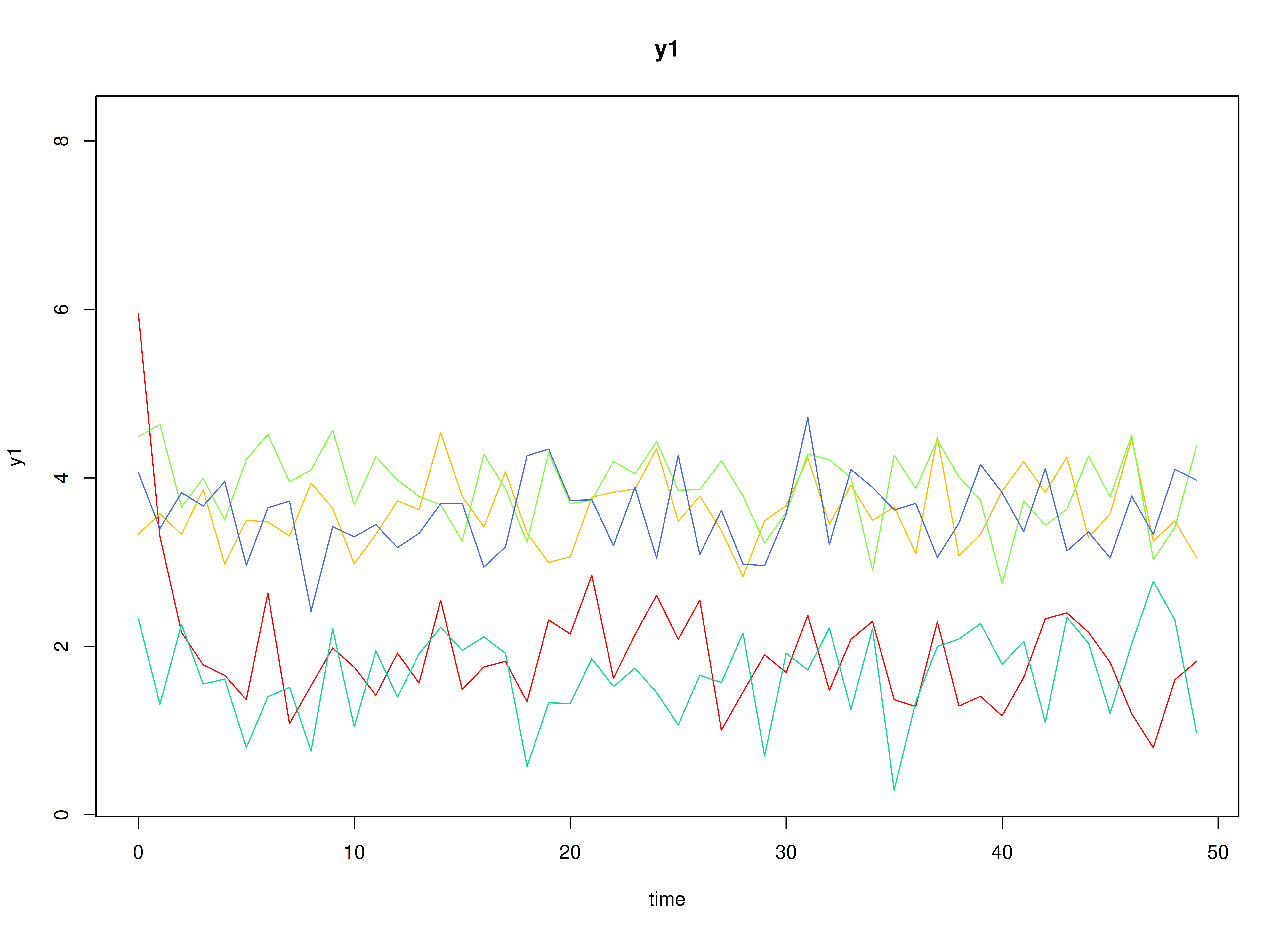

Visualizing the Dynamics Without Process Noise (n = 5 with Different Initial Condition)

Using the SimSSMIVary Function from the simStateSpace Package to Simulate Data

library(simStateSpace)
sim <- SimSSMIVary(
  n = n,
  time = time,
  mu0 = mu0,
  sigma0_l = sigma0_l,
  alpha = alpha,
  beta = beta,
  psi_l = psi_l,
  nu = nu,
  lambda = lambda,
  theta_l = theta_l
)
data <- as.data.frame(sim)
head(data)
#>   id time       y1       y2
#> 1  1    0 3.040533 3.202203
#> 2  1    1 3.630653 4.691667
#> 3  1    2 2.621350 5.240797
#> 4  1    3 2.073843 5.555230
#> 5  1    4 2.013430 5.269451
#> 6  1    5 1.677296 2.836631
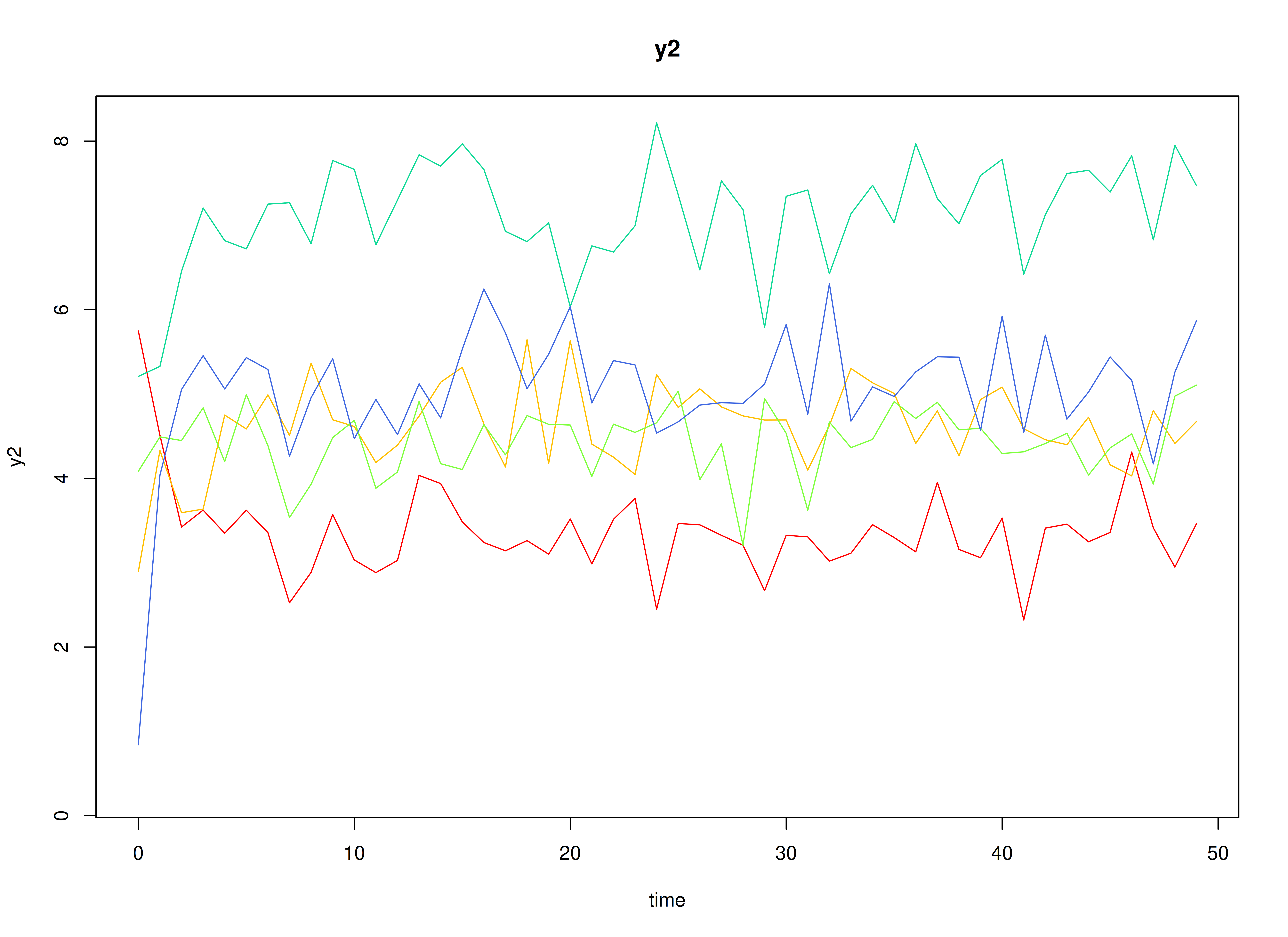
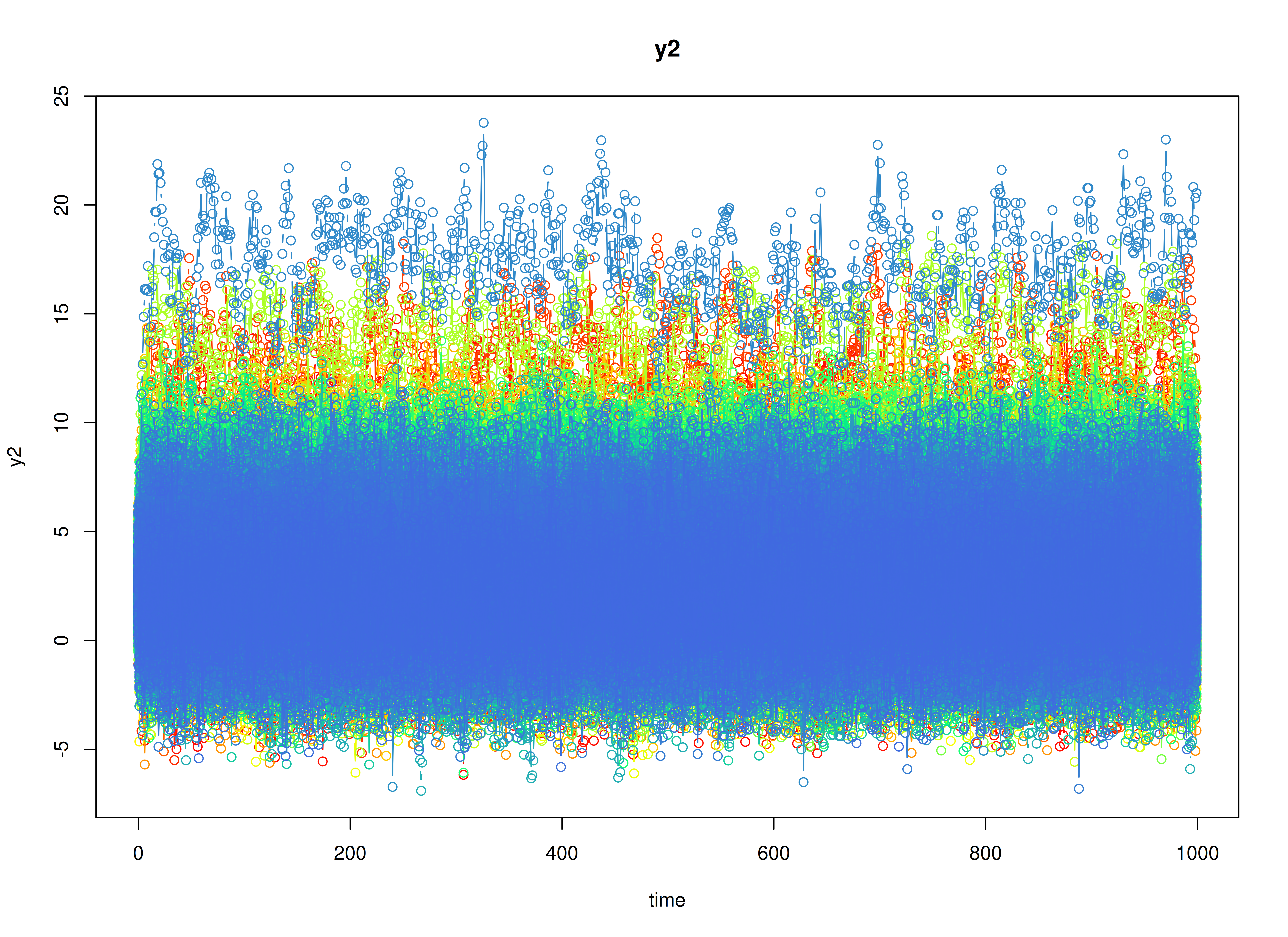
plot(sim)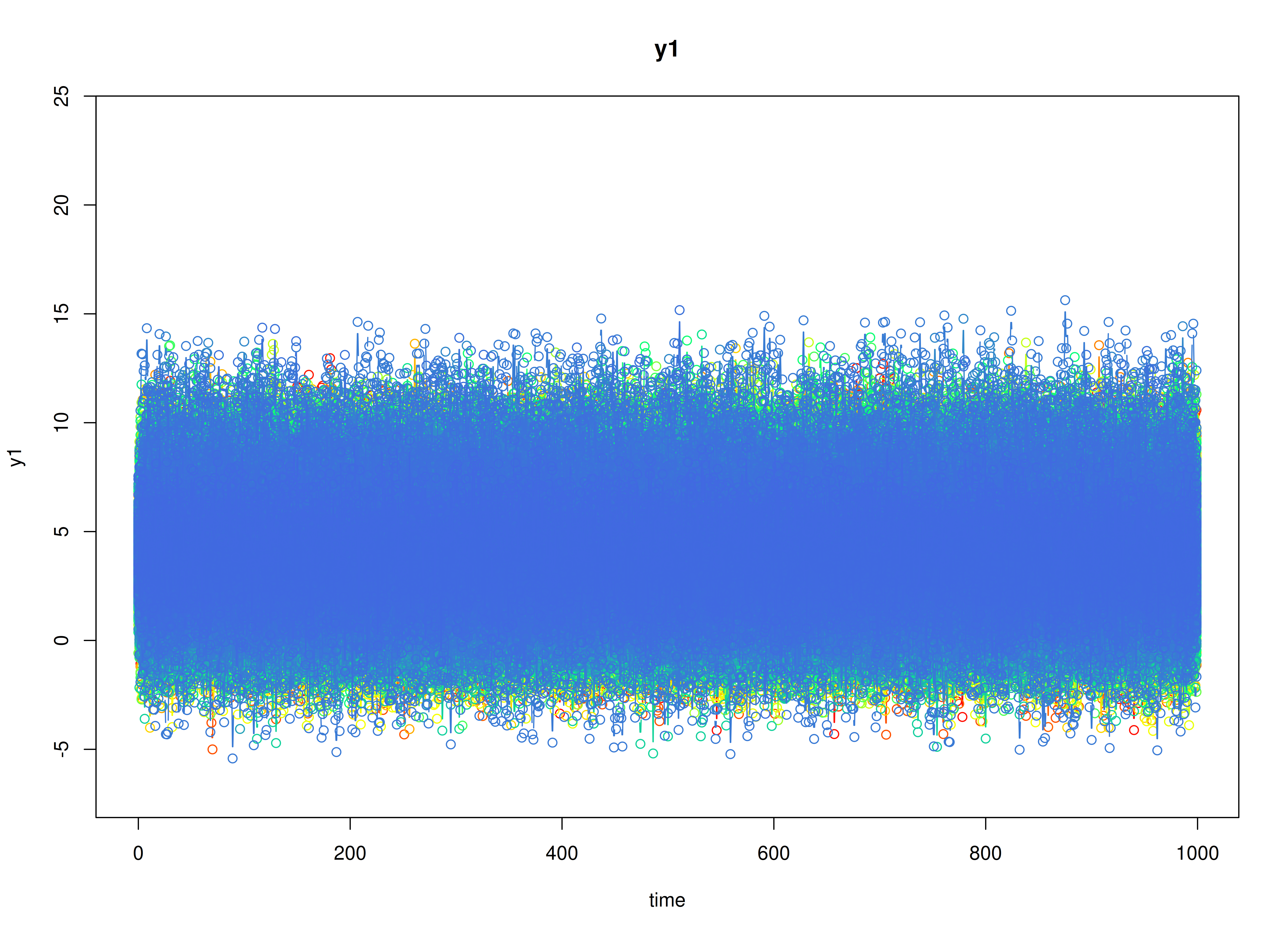

Model Fitting

The FitDTVARIDMx function fits a DT-VAR model on each individual $i$.

library(fitDTVARMx)
fit <- FitDTVARIDMx(
  data = data,
  observed = paste0("y", seq_len(k)),
  id = "id",
  mu0_values = mu0[[1]],
  sigma0_l_values = sigma0_l,
  ncores = parallel::detectCores()
)
#> Error in sigma0_l_values %*% t(sigma0_l_values): requires numeric/complex matrix/vector arguments
summary(fit, means = FALSE)
#> Error: object 'fit' not found
summary(fit, means = TRUE)
#> Error: object 'fit' not found

References

Bringmann, L. F., Vissers, N., Wichers, M., Geschwind, N., Kuppens, P., Peeters, F., Borsboom, D., & Tuerlinckx, F. (2013). A network approach to psychopathology: New insights into clinical longitudinal data. PLoS ONE, 8(4). https://doi.org/10.1371/journal.pone.0060188

Hunter, M. D. (2017). State space modeling in an open source, modular, structural equation modeling environment. Structural Equation Modeling: A Multidisciplinary Journal, 25(2), 307–324. https://doi.org/10.1080/10705511.2017.1369354

Neale, M. C., Hunter, M. D., Pritikin, J. N., Zahery, M., Brick, T. R., Kirkpatrick, R. M., Estabrook, R., Bates, T. C., Maes, H. H., & Boker, S. M. (2015). OpenMx 2.0: Extended structural equation and statistical modeling. Psychometrika, 81(2), 535–549. https://doi.org/10.1007/s11336-014-9435-8

R Core Team. (2024). R: A language and environment for statistical computing. R Foundation for Statistical Computing. https://www.R-project.org/