Delta Method Sampling Variance-Covariance Matrix for the Standardized Indirect Effect Centrality Over a Specific Time Interval or a Range of Time Intervals
Source:R/cTMed-delta-indirect-central-std.R
DeltaIndirectCentralStd.RdThis function computes the delta method sampling variance-covariance matrix for the standardized indirect effect centrality over a specific time interval \(\Delta t\) or a range of time intervals using the first-order stochastic differential equation model's drift matrix \(\boldsymbol{\Phi}\) and process noise covariance matrix \(\boldsymbol{\Sigma}\).
Usage
DeltaIndirectCentralStd(
  phi,
  sigma,
  vcov_theta,
  delta_t,
  sigma_diag = FALSE,
  ncores = NULL,
  tol = 0.001
)
Arguments
- phi
Numeric matrix. The drift matrix (\(\boldsymbol{\Phi}\)).
phishould have row and column names pertaining to the variables in the system.- sigma
Numeric matrix. The process noise covariance matrix (\(\boldsymbol{\Sigma}\)).
- vcov_theta
Numeric matrix. The sampling variance-covariance matrix of \(\mathrm{vec} \left( \boldsymbol{\Phi} \right)\) and \(\mathrm{vech} \left( \boldsymbol{\Sigma} \right)\)
- delta_t
Vector of positive numbers. Time interval (\(\Delta t\)).
- sigma_diag
Logical. If
sigma_diag = TRUE, treat \(\boldsymbol{\Sigma}\) as a diagonal matrix.- ncores
Positive integer. Number of cores to use. If
ncores = NULL, use a single core. Consider using multiple cores when the length ofdelta_tis long.- tol
Numeric. Smallest possible time interval to allow.
Value
Returns an object
of class ctmeddelta which is a list with the following elements:
- call
Function call.
- args
Function arguments.
- fun
Function used ("DeltaIndirectCentralStd").
- output
A list of length
length(delta_t).
Each element in the output list has the following elements:
- delta_t
Time interval.
- jacobian
Jacobian matrix.
- est
Estimated standardized indirect effect centrality.
- vcov
Sampling variance-covariance matrix of estimated standardized indirect effect centrality.
Details
See IndirectCentralStd() for more details.
Delta Method
Let \(\boldsymbol{\theta}\) be a vector that combines \(\mathrm{vec} \left( \boldsymbol{\Phi} \right)\), that is, the elements of the \(\boldsymbol{\Phi}\) matrix in vector form sorted column-wise and \(\mathrm{vech} \left( \boldsymbol{\Sigma} \right)\), that is, the unique elements of the \(\boldsymbol{\Sigma}\) matrix in vector form sorted column-wise. Let \(\hat{\boldsymbol{\theta}}\) be a vector that combines \(\mathrm{vec} \left( \hat{\boldsymbol{\Phi}} \right)\) and \(\mathrm{vech} \left( \hat{\boldsymbol{\Sigma}} \right)\). By the multivariate central limit theory, the function \(\mathbf{g}\) using \(\hat{\boldsymbol{\theta}}\) as input can be expressed as:
$$ \sqrt{n} \left( \mathbf{g} \left( \hat{\boldsymbol{\theta}} \right) - \mathbf{g} \left( \boldsymbol{\theta} \right) \right) \xrightarrow[]{ \mathrm{D} } \mathcal{N} \left( 0, \mathbf{J} \boldsymbol{\Gamma} \mathbf{J}^{\prime} \right) $$
where \(\mathbf{J}\) is the matrix of first-order derivatives of the function \(\mathbf{g}\) with respect to the elements of \(\boldsymbol{\theta}\) and \(\boldsymbol{\Gamma}\) is the asymptotic variance-covariance matrix of \(\hat{\boldsymbol{\theta}}\).
From the former, we can derive the distribution of \(\mathbf{g} \left( \hat{\boldsymbol{\theta}} \right)\) as follows:
$$ \mathbf{g} \left( \hat{\boldsymbol{\theta}} \right) \approx \mathcal{N} \left( \mathbf{g} \left( \boldsymbol{\theta} \right) , n^{-1} \mathbf{J} \boldsymbol{\Gamma} \mathbf{J}^{\prime} \right) $$
The uncertainty associated with the estimator \(\mathbf{g} \left( \hat{\boldsymbol{\theta}} \right)\) is, therefore, given by \(n^{-1} \mathbf{J} \boldsymbol{\Gamma} \mathbf{J}^{\prime}\) . When \(\boldsymbol{\Gamma}\) is unknown, by substitution, we can use the estimated sampling variance-covariance matrix of \(\hat{\boldsymbol{\theta}}\), that is, \(\hat{\mathbb{V}} \left( \hat{\boldsymbol{\theta}} \right)\) for \(n^{-1} \boldsymbol{\Gamma}\). Therefore, the sampling variance-covariance matrix of \(\mathbf{g} \left( \hat{\boldsymbol{\theta}} \right)\) is given by
$$ \mathbf{g} \left( \hat{\boldsymbol{\theta}} \right) \approx \mathcal{N} \left( \mathbf{g} \left( \boldsymbol{\theta} \right) , \mathbf{J} \hat{\mathbb{V}} \left( \hat{\boldsymbol{\theta}} \right) \mathbf{J}^{\prime} \right) . $$
References
Bollen, K. A. (1987). Total, direct, and indirect effects in structural equation models. Sociological Methodology, 17, 37. doi:10.2307/271028
Deboeck, P. R., & Preacher, K. J. (2015). No need to be discrete: A method for continuous time mediation analysis. Structural Equation Modeling: A Multidisciplinary Journal, 23 (1), 61-75. doi:10.1080/10705511.2014.973960
Pesigan, I. J. A., Russell, M. A., & Chow, S.-M. (2025). Inferences and effect sizes for direct, indirect, and total effects in continuous-time mediation models. Psychological Methods. doi:10.1037/met0000779
Ryan, O., & Hamaker, E. L. (2021). Time to intervene: A continuous-time approach to network analysis and centrality. Psychometrika, 87 (1), 214-252. doi:10.1007/s11336-021-09767-0
Examples
phi <- matrix(
data = c(
-0.357, 0.771, -0.450,
0.0, -0.511, 0.729,
0, 0, -0.693
),
nrow = 3
)
colnames(phi) <- rownames(phi) <- c("x", "m", "y")
sigma <- matrix(
data = c(
0.24455556, 0.02201587, -0.05004762,
0.02201587, 0.07067800, 0.01539456,
-0.05004762, 0.01539456, 0.07553061
),
nrow = 3
)
vcov_theta <- matrix(
data = c(
0.00843, 0.00040, -0.00151, -0.00600, -0.00033,
0.00110, 0.00324, 0.00020, -0.00061, -0.00115,
0.00011, 0.00015, 0.00001, -0.00002, -0.00001,
0.00040, 0.00374, 0.00016, -0.00022, -0.00273,
-0.00016, 0.00009, 0.00150, 0.00012, -0.00010,
-0.00026, 0.00002, 0.00012, 0.00004, -0.00001,
-0.00151, 0.00016, 0.00389, 0.00103, -0.00007,
-0.00283, -0.00050, 0.00000, 0.00156, 0.00021,
-0.00005, -0.00031, 0.00001, 0.00007, 0.00006,
-0.00600, -0.00022, 0.00103, 0.00644, 0.00031,
-0.00119, -0.00374, -0.00021, 0.00070, 0.00064,
-0.00015, -0.00005, 0.00000, 0.00003, -0.00001,
-0.00033, -0.00273, -0.00007, 0.00031, 0.00287,
0.00013, -0.00014, -0.00170, -0.00012, 0.00006,
0.00014, -0.00001, -0.00015, 0.00000, 0.00001,
0.00110, -0.00016, -0.00283, -0.00119, 0.00013,
0.00297, 0.00063, -0.00004, -0.00177, -0.00013,
0.00005, 0.00017, -0.00002, -0.00008, 0.00001,
0.00324, 0.00009, -0.00050, -0.00374, -0.00014,
0.00063, 0.00495, 0.00024, -0.00093, -0.00020,
0.00006, -0.00010, 0.00000, -0.00001, 0.00004,
0.00020, 0.00150, 0.00000, -0.00021, -0.00170,
-0.00004, 0.00024, 0.00214, 0.00012, -0.00002,
-0.00004, 0.00000, 0.00006, -0.00005, -0.00001,
-0.00061, 0.00012, 0.00156, 0.00070, -0.00012,
-0.00177, -0.00093, 0.00012, 0.00223, 0.00004,
-0.00002, -0.00003, 0.00001, 0.00003, -0.00013,
-0.00115, -0.00010, 0.00021, 0.00064, 0.00006,
-0.00013, -0.00020, -0.00002, 0.00004, 0.00057,
0.00001, -0.00009, 0.00000, 0.00000, 0.00001,
0.00011, -0.00026, -0.00005, -0.00015, 0.00014,
0.00005, 0.00006, -0.00004, -0.00002, 0.00001,
0.00012, 0.00001, 0.00000, -0.00002, 0.00000,
0.00015, 0.00002, -0.00031, -0.00005, -0.00001,
0.00017, -0.00010, 0.00000, -0.00003, -0.00009,
0.00001, 0.00014, 0.00000, 0.00000, -0.00005,
0.00001, 0.00012, 0.00001, 0.00000, -0.00015,
-0.00002, 0.00000, 0.00006, 0.00001, 0.00000,
0.00000, 0.00000, 0.00010, 0.00001, 0.00000,
-0.00002, 0.00004, 0.00007, 0.00003, 0.00000,
-0.00008, -0.00001, -0.00005, 0.00003, 0.00000,
-0.00002, 0.00000, 0.00001, 0.00005, 0.00001,
-0.00001, -0.00001, 0.00006, -0.00001, 0.00001,
0.00001, 0.00004, -0.00001, -0.00013, 0.00001,
0.00000, -0.00005, 0.00000, 0.00001, 0.00012
),
nrow = 15
)
# Specific time interval ----------------------------------------------------
DeltaIndirectCentralStd(
phi = phi,
sigma = sigma,
vcov_theta = vcov_theta,
delta_t = 1
)
#> Call:
#> DeltaIndirectCentralStd(phi = phi, sigma = sigma, vcov_theta = vcov_theta,
#> delta_t = 1)
#>
#> Indirect Effect Centrality
#> variable interval est se z p 2.5% 97.5%
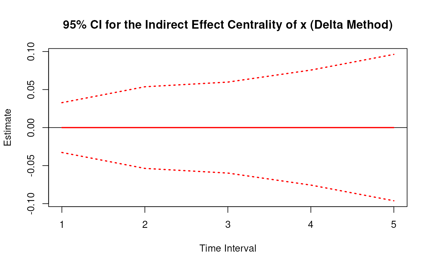
#> 1 x 1 0.0000 0.0167 0.0000 1 -0.0327 0.0327
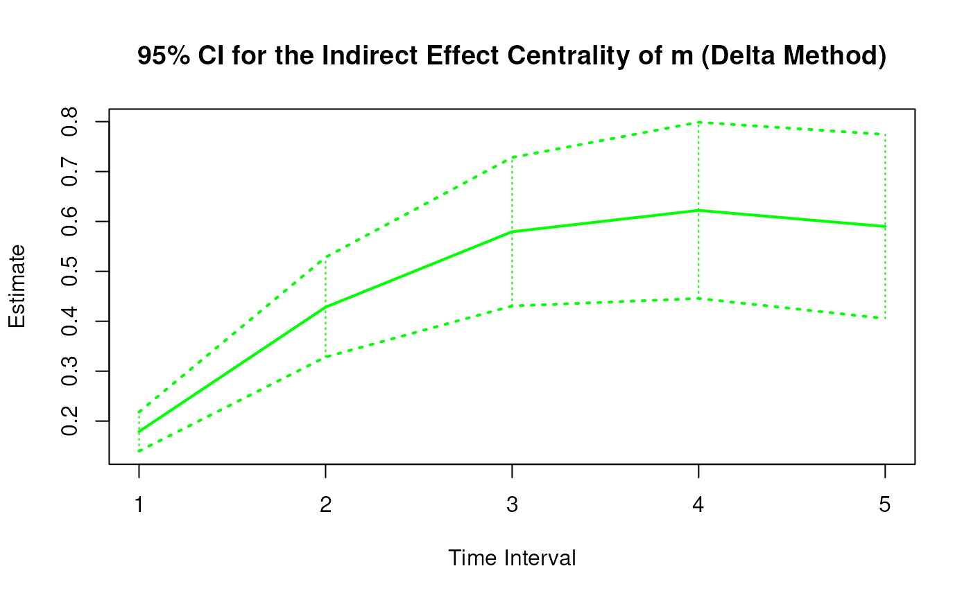
#> 2 m 1 0.1789 0.0200 8.9504 0 0.1397 0.2181
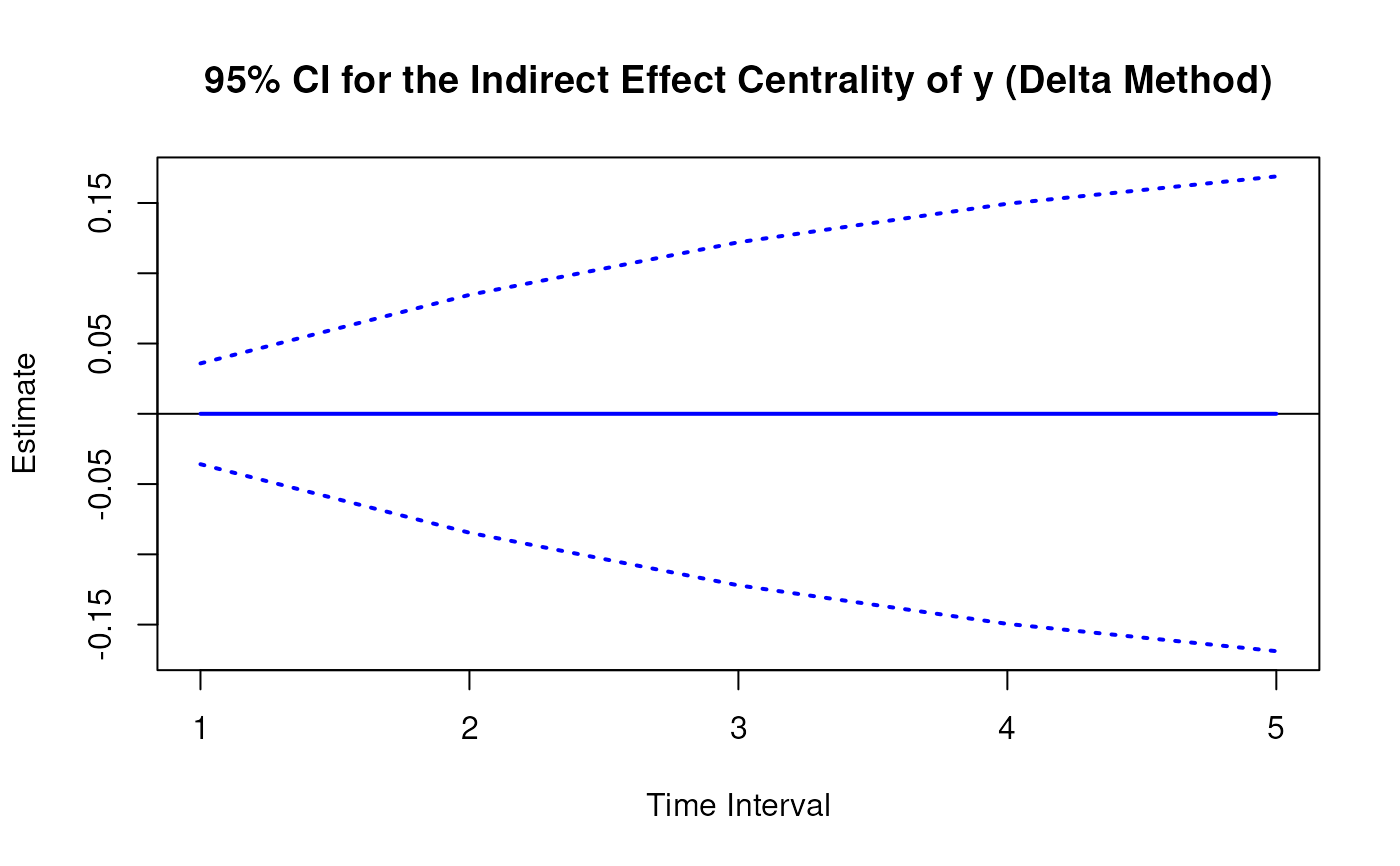
#> 3 y 1 0.0000 0.0183 0.0000 1 -0.0359 0.0359
# Range of time intervals ---------------------------------------------------
delta <- DeltaIndirectCentralStd(
phi = phi,
sigma = sigma,
vcov_theta = vcov_theta,
delta_t = 1:5
)
plot(delta)

 # Methods -------------------------------------------------------------------
# DeltaIndirectCentralStd has a number of methods including
# print, summary, confint, and plot
print(delta)
#> Call:
#> DeltaIndirectCentralStd(phi = phi, sigma = sigma, vcov_theta = vcov_theta,
#> delta_t = 1:5)
#>
#> Indirect Effect Centrality
#> variable interval est se z p 2.5% 97.5%
#> 1 x 1 0.0000 0.0167 0.0000 1 -0.0327 0.0327
#> 2 m 1 0.1789 0.0200 8.9504 0 0.1397 0.2181
#> 3 y 1 0.0000 0.0183 0.0000 1 -0.0359 0.0359
#> 4 x 2 0.0000 0.0274 0.0000 1 -0.0537 0.0537
#> 5 m 2 0.4283 0.0510 8.3988 0 0.3283 0.5282
#> 6 y 2 0.0000 0.0432 0.0000 1 -0.0846 0.0846
#> 7 x 3 0.0000 0.0305 0.0000 1 -0.0598 0.0598
#> 8 m 3 0.5794 0.0759 7.6315 0 0.4306 0.7282
#> 9 y 3 0.0000 0.0623 0.0000 1 -0.1221 0.1221
#> 10 x 4 0.0000 0.0386 0.0000 1 -0.0756 0.0756
#> 11 m 4 0.6222 0.0901 6.9059 0 0.4456 0.7988
#> 12 y 4 0.0000 0.0763 0.0000 1 -0.1495 0.1495
#> 13 x 5 0.0000 0.0491 0.0000 1 -0.0962 0.0962
#> 14 m 5 0.5899 0.0941 6.2696 0 0.4055 0.7744
#> 15 y 5 0.0000 0.0862 0.0000 1 -0.1689 0.1689
summary(delta)
#> Call:
#> DeltaIndirectCentralStd(phi = phi, sigma = sigma, vcov_theta = vcov_theta,
#> delta_t = 1:5)
#>
#> Indirect Effect Centrality
#> variable interval est se z p 2.5% 97.5%
#> 1 x 1 0.0000 0.0167 0.0000 1 -0.0327 0.0327
#> 2 m 1 0.1789 0.0200 8.9504 0 0.1397 0.2181
#> 3 y 1 0.0000 0.0183 0.0000 1 -0.0359 0.0359
#> 4 x 2 0.0000 0.0274 0.0000 1 -0.0537 0.0537
#> 5 m 2 0.4283 0.0510 8.3988 0 0.3283 0.5282
#> 6 y 2 0.0000 0.0432 0.0000 1 -0.0846 0.0846
#> 7 x 3 0.0000 0.0305 0.0000 1 -0.0598 0.0598
#> 8 m 3 0.5794 0.0759 7.6315 0 0.4306 0.7282
#> 9 y 3 0.0000 0.0623 0.0000 1 -0.1221 0.1221
#> 10 x 4 0.0000 0.0386 0.0000 1 -0.0756 0.0756
#> 11 m 4 0.6222 0.0901 6.9059 0 0.4456 0.7988
#> 12 y 4 0.0000 0.0763 0.0000 1 -0.1495 0.1495
#> 13 x 5 0.0000 0.0491 0.0000 1 -0.0962 0.0962
#> 14 m 5 0.5899 0.0941 6.2696 0 0.4055 0.7744
#> 15 y 5 0.0000 0.0862 0.0000 1 -0.1689 0.1689
confint(delta, level = 0.95)
#> variable interval 2.5 % 97.5 %
#> 1 x 1 -0.03273421 0.03273421
#> 2 m 1 0.13971515 0.21806096
#> 3 y 1 -0.03587065 0.03587065
#> 4 x 2 -0.05367710 0.05367710
#> 5 m 2 0.32832799 0.52821273
#> 6 y 2 -0.08462271 0.08462271
#> 7 x 3 -0.05981430 0.05981430
#> 8 m 3 0.43060735 0.72822429
#> 9 y 3 -0.12205363 0.12205363
#> 10 x 4 -0.07562045 0.07562045
#> 11 m 4 0.44562892 0.79881634
#> 12 y 4 -0.14948781 0.14948781
#> 13 x 5 -0.09623650 0.09623650
#> 14 m 5 0.40551136 0.77435334
#> 15 y 5 -0.16889898 0.16889898
plot(delta)
# Methods -------------------------------------------------------------------
# DeltaIndirectCentralStd has a number of methods including
# print, summary, confint, and plot
print(delta)
#> Call:
#> DeltaIndirectCentralStd(phi = phi, sigma = sigma, vcov_theta = vcov_theta,
#> delta_t = 1:5)
#>
#> Indirect Effect Centrality
#> variable interval est se z p 2.5% 97.5%
#> 1 x 1 0.0000 0.0167 0.0000 1 -0.0327 0.0327
#> 2 m 1 0.1789 0.0200 8.9504 0 0.1397 0.2181
#> 3 y 1 0.0000 0.0183 0.0000 1 -0.0359 0.0359
#> 4 x 2 0.0000 0.0274 0.0000 1 -0.0537 0.0537
#> 5 m 2 0.4283 0.0510 8.3988 0 0.3283 0.5282
#> 6 y 2 0.0000 0.0432 0.0000 1 -0.0846 0.0846
#> 7 x 3 0.0000 0.0305 0.0000 1 -0.0598 0.0598
#> 8 m 3 0.5794 0.0759 7.6315 0 0.4306 0.7282
#> 9 y 3 0.0000 0.0623 0.0000 1 -0.1221 0.1221
#> 10 x 4 0.0000 0.0386 0.0000 1 -0.0756 0.0756
#> 11 m 4 0.6222 0.0901 6.9059 0 0.4456 0.7988
#> 12 y 4 0.0000 0.0763 0.0000 1 -0.1495 0.1495
#> 13 x 5 0.0000 0.0491 0.0000 1 -0.0962 0.0962
#> 14 m 5 0.5899 0.0941 6.2696 0 0.4055 0.7744
#> 15 y 5 0.0000 0.0862 0.0000 1 -0.1689 0.1689
summary(delta)
#> Call:
#> DeltaIndirectCentralStd(phi = phi, sigma = sigma, vcov_theta = vcov_theta,
#> delta_t = 1:5)
#>
#> Indirect Effect Centrality
#> variable interval est se z p 2.5% 97.5%
#> 1 x 1 0.0000 0.0167 0.0000 1 -0.0327 0.0327
#> 2 m 1 0.1789 0.0200 8.9504 0 0.1397 0.2181
#> 3 y 1 0.0000 0.0183 0.0000 1 -0.0359 0.0359
#> 4 x 2 0.0000 0.0274 0.0000 1 -0.0537 0.0537
#> 5 m 2 0.4283 0.0510 8.3988 0 0.3283 0.5282
#> 6 y 2 0.0000 0.0432 0.0000 1 -0.0846 0.0846
#> 7 x 3 0.0000 0.0305 0.0000 1 -0.0598 0.0598
#> 8 m 3 0.5794 0.0759 7.6315 0 0.4306 0.7282
#> 9 y 3 0.0000 0.0623 0.0000 1 -0.1221 0.1221
#> 10 x 4 0.0000 0.0386 0.0000 1 -0.0756 0.0756
#> 11 m 4 0.6222 0.0901 6.9059 0 0.4456 0.7988
#> 12 y 4 0.0000 0.0763 0.0000 1 -0.1495 0.1495
#> 13 x 5 0.0000 0.0491 0.0000 1 -0.0962 0.0962
#> 14 m 5 0.5899 0.0941 6.2696 0 0.4055 0.7744
#> 15 y 5 0.0000 0.0862 0.0000 1 -0.1689 0.1689
confint(delta, level = 0.95)
#> variable interval 2.5 % 97.5 %
#> 1 x 1 -0.03273421 0.03273421
#> 2 m 1 0.13971515 0.21806096
#> 3 y 1 -0.03587065 0.03587065
#> 4 x 2 -0.05367710 0.05367710
#> 5 m 2 0.32832799 0.52821273
#> 6 y 2 -0.08462271 0.08462271
#> 7 x 3 -0.05981430 0.05981430
#> 8 m 3 0.43060735 0.72822429
#> 9 y 3 -0.12205363 0.12205363
#> 10 x 4 -0.07562045 0.07562045
#> 11 m 4 0.44562892 0.79881634
#> 12 y 4 -0.14948781 0.14948781
#> 13 x 5 -0.09623650 0.09623650
#> 14 m 5 0.40551136 0.77435334
#> 15 y 5 -0.16889898 0.16889898
plot(delta)

 #' @family Continuous-Time Mediation Functions