Total and Indirect Effect Centrality in Continuous-Time Mediation Model (Bootstrap)

The cTMed package provides a bootstrap approach, in addition to the delta and Monte Carlo methods, for estimating and quantifying uncertainty in total and indirect effect centrality within continuous-time mediation models across different time intervals. This vignette shows both unstandardized and standardized effect centrality using bootstrap samples of the drift matrix and, for standardized centrality, the process noise covariance matrix.

In this example, we will use the fitted model from Fit the Continuous-Time Vector Autoregressive Model Using the dynr Package. The object fit represents a fitted CT-VAR model created using the dynr package.

summary(fit)
#> Coefficients:
#>             Estimate Std. Error t value  ci.lower  ci.upper Pr(>|t|)
#> phi_1_1    -0.351839   0.036416  -9.662 -0.423213 -0.280465   <2e-16 ***
#> phi_2_1     0.744282   0.021777  34.177  0.701599  0.786964   <2e-16 ***
#> phi_3_1    -0.458680   0.023534 -19.490 -0.504806 -0.412554   <2e-16 ***
#> phi_1_2     0.017311   0.031705   0.546 -0.044829  0.079451   0.2925
#> phi_2_2    -0.488821   0.019277 -25.358 -0.526602 -0.451039   <2e-16 ***
#> phi_3_2     0.726800   0.020871  34.824  0.685894  0.767706   <2e-16 ***
#> phi_1_3    -0.023814   0.024025  -0.991 -0.070903  0.023275   0.1608
#> phi_2_3    -0.009810   0.014718  -0.667 -0.038657  0.019036   0.2525
#> phi_3_3    -0.688334   0.016040 -42.913 -0.719773 -0.656896   <2e-16 ***
#> sigma_1_1   0.242180   0.006794  35.646  0.228864  0.255496   <2e-16 ***
#> sigma_2_1   0.023273   0.002545   9.146  0.018285  0.028261   <2e-16 ***
#> sigma_3_1  -0.050574   0.002749 -18.395 -0.055963 -0.045186   <2e-16 ***
#> sigma_2_2   0.070722   0.001907  37.093  0.066985  0.074458   <2e-16 ***
#> sigma_3_2   0.014987   0.001381  10.854  0.012281  0.017694   <2e-16 ***
#> sigma_3_3   0.072376   0.002099  34.475  0.068261  0.076491   <2e-16 ***
#> theta_1_1   0.198861   0.001170 169.909  0.196567  0.201155   <2e-16 ***
#> theta_2_2   0.199520   0.001000 199.500  0.197560  0.201480   <2e-16 ***
#> theta_3_3   0.201172   0.001016 198.052  0.199181  0.203162   <2e-16 ***
#> mu0_1_1     0.006324   0.111110   0.057 -0.211447  0.224095   0.4773
#> mu0_2_1    -0.042530   0.114320  -0.372 -0.266593  0.181533   0.3549
#> mu0_3_1     0.130043   0.102109   1.274 -0.070086  0.330172   0.1014
#> sigma0_1_1  1.150287   0.168811   6.814  0.819425  1.481150   <2e-16 ***
#> sigma0_2_1  0.413648   0.133495   3.099  0.152003  0.675293   0.0010 ***
#> sigma0_3_1  0.225993   0.123478   1.830 -0.016019  0.468006   0.0336 *
#> sigma0_2_2  1.221957   0.182233   6.705  0.864787  1.579128   <2e-16 ***
#> sigma0_3_2  0.235327   0.117629   2.001  0.004779  0.465875   0.0227 *
#> sigma0_3_3  0.962594   0.142152   6.772  0.683981  1.241207   <2e-16 ***
#> ---
#> Signif. codes:  0 '***' 0.001 '**' 0.01 '*' 0.05 '.' 0.1 ' ' 1
#>
#> -2 log-likelihood value at convergence = 429365.49
#> AIC = 429419.49
#> BIC = 429676.34

We need to extract the estimated parameters from the fitted object, which will be used to generate bootstrap samples.

est <- coef(fit)
n
#> [1] 100
time
#> [1] 1000
delta_t
#> [1] 0.1
lambda
#>      [,1] [,2] [,3]
#> [1,]    1    0    0
#> [2,]    0    1    0
#> [3,]    0    0    1
nu
#> [1] 0 0 0
mu
#> [1] 0 0 0
mu0 <- est[
  c(
    "mu0_1_1",
    "mu0_2_1",
    "mu0_3_1"
  )
]
mu0
#>      mu0_1_1      mu0_2_1      mu0_3_1
#>  0.006324029 -0.042529883  0.130043337
sigma0 <- matrix(
  data = est[
    c(
      "sigma0_1_1",
      "sigma0_2_1",
      "sigma0_3_1",
      "sigma0_2_1",
      "sigma0_2_2",
      "sigma0_3_2",
      "sigma0_3_1",
      "sigma0_3_2",
      "sigma0_3_3"
    )
  ],
  nrow = 3,
  ncol = 3
)
sigma0
#>           [,1]      [,2]      [,3]
#> [1,] 1.1502873 0.4136480 0.2259932
#> [2,] 0.4136480 1.2219574 0.2353267
#> [3,] 0.2259932 0.2353267 0.9625940
sigma0_l <- t(chol(sigma0))
phi <- matrix(
  data = est[
    c(
      "phi_1_1",
      "phi_2_1",
      "phi_3_1",
      "phi_1_2",
      "phi_2_2",
      "phi_3_2",
      "phi_1_3",
      "phi_2_3",
      "phi_3_3"
    )
  ],
  nrow = 3,
  ncol = 3
)
phi
#>            [,1]        [,2]         [,3]
#> [1,] -0.3518392  0.01731083 -0.023814339
#> [2,]  0.7442816 -0.48882067 -0.009810166
#> [3,] -0.4586796  0.72679980 -0.688334177
sigma <- matrix(
  data = est[
    c(
      "sigma_1_1", "sigma_2_1", "sigma_3_1",
      "sigma_2_1", "sigma_2_2", "sigma_3_2",
      "sigma_3_1", "sigma_3_2", "sigma_3_3"
    )
  ],
  nrow = 3,
  ncol = 3
)
sigma
#>             [,1]       [,2]        [,3]
#> [1,]  0.24218026 0.02327296 -0.05057416
#> [2,]  0.02327296 0.07072156  0.01498732
#> [3,] -0.05057416 0.01498732  0.07237598
sigma_l <- t(chol(sigma))
theta <- diag(3)
diag(theta) <- est[
  c(
    "theta_1_1",
    "theta_2_2",
    "theta_3_3"
  )
]
theta
#>           [,1]      [,2]      [,3]
#> [1,] 0.1988611 0.0000000 0.0000000
#> [2,] 0.0000000 0.1995203 0.0000000
#> [3,] 0.0000000 0.0000000 0.2011716
theta_l <- t(chol(theta))

R <- 200L # use at least 1000 in actual research
path <- getwd()
prefix <- "ou"

The estimated parameters are then passed as arguments to the PBSSMOUFixed function from the bootStateSpace package, which generates a parametric bootstrap sampling distribution of the parameter estimates. The argument R specifies the number of bootstrap replications. The generated data and model estimates are stored in path using the specified prefix for the file names. The ncores = parallel::detectCores() argument instructs the function to use all available CPU cores in the system.

NOTE: Fitting the CT-VAR model multiple times is computationally intensive.

library(bootStateSpace)
boot <- PBSSMOUFixed(
  R = R,
  path = path,
  prefix = prefix,
  n = n,
  time = time,
  delta_t = delta_t,
  mu0 = mu0,
  sigma0_l = sigma0_l,
  mu = mu,
  phi = phi,
  sigma_l = sigma_l,
  nu = nu,
  lambda = lambda,
  theta_l = theta_l,
  ncores = parallel::detectCores(),
  seed = 42,
  clean = FALSE
)

The extract function from the bootStateSpace package is used to extract the bootstrap phi matrices as well as the sigma matrices.

phi <- extract(object = boot, what = "phi")

sigma <- extract(object = boot, what = "sigma")

In this example, we calculate total and indirect effect centrality for the variables x, m, and y over time intervals ranging from 0 to 10. Unlike the path-specific mediation functions, the centrality functions do not require from, to, or med arguments because centrality is computed for each variable in the dynamic system.

# time intervals
delta_t <- seq(from = 0, to = 10, length.out = 1000)

We also need the estimated drift matrix from the original sample.

# estimated drift matrix
phi_hat <- matrix(
  data = est[
    c(
      "phi_1_1",
      "phi_2_1",
      "phi_3_1",
      "phi_1_2",
      "phi_2_2",
      "phi_3_2",
      "phi_1_3",
      "phi_2_3",
      "phi_3_3"
    )
  ],
  nrow = 3,
  ncol = 3
)
colnames(phi_hat) <- rownames(phi_hat) <- c("x", "m", "y")

For the standardized centrality estimates, the estimated process noise covariance matrix from the original sample is also needed.

# estimated process noise covariance matrix
sigma_hat <- matrix(
  data = est[
    c(
      "sigma_1_1", "sigma_2_1", "sigma_3_1",
      "sigma_2_1", "sigma_2_2", "sigma_3_2",
      "sigma_3_1", "sigma_3_2", "sigma_3_3"
    )
  ],
  nrow = 3,
  ncol = 3
)
colnames(sigma_hat) <- rownames(sigma_hat) <- c("x", "m", "y")

Bootstrap Method: Unstandardized Centrality

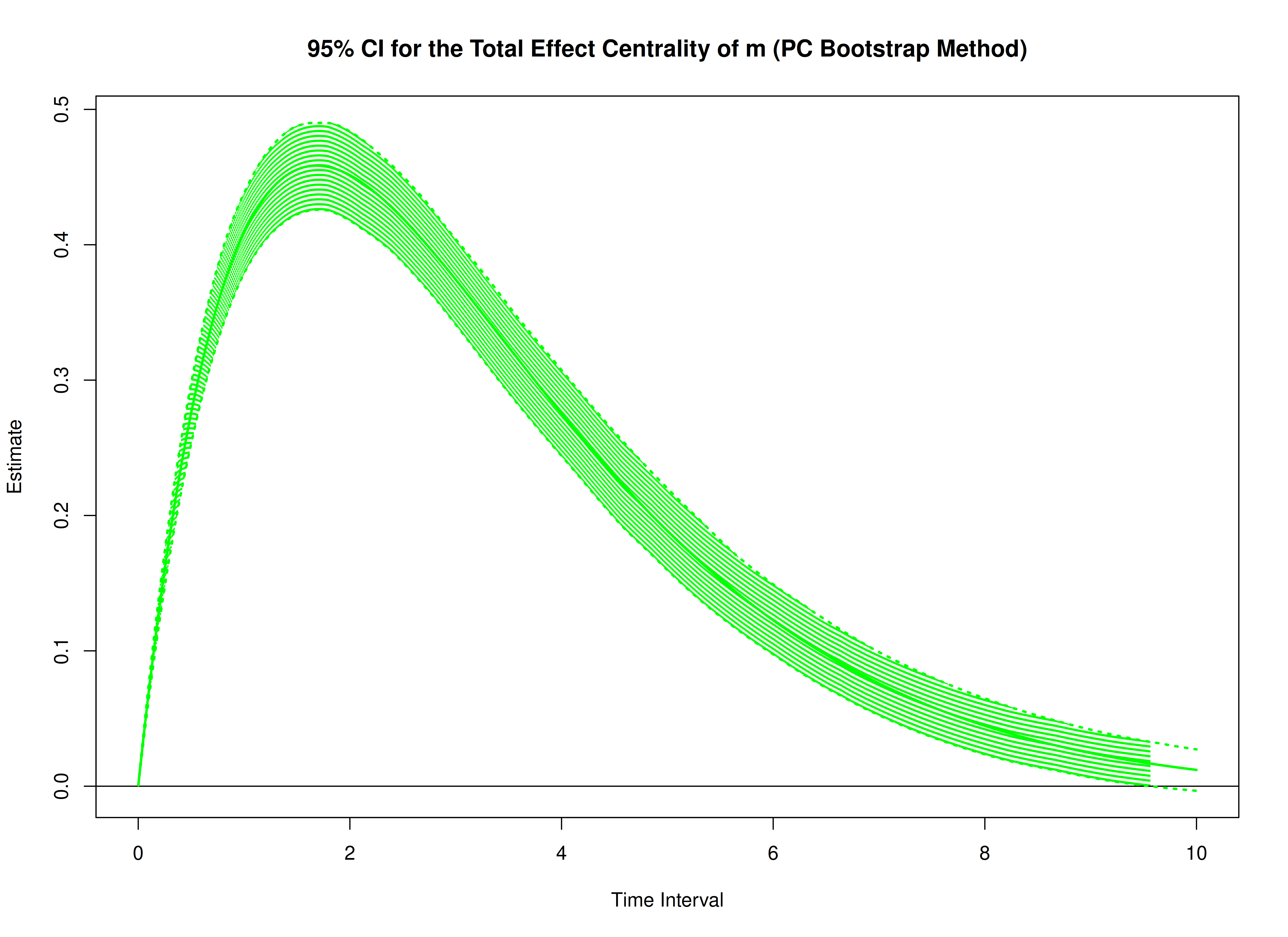
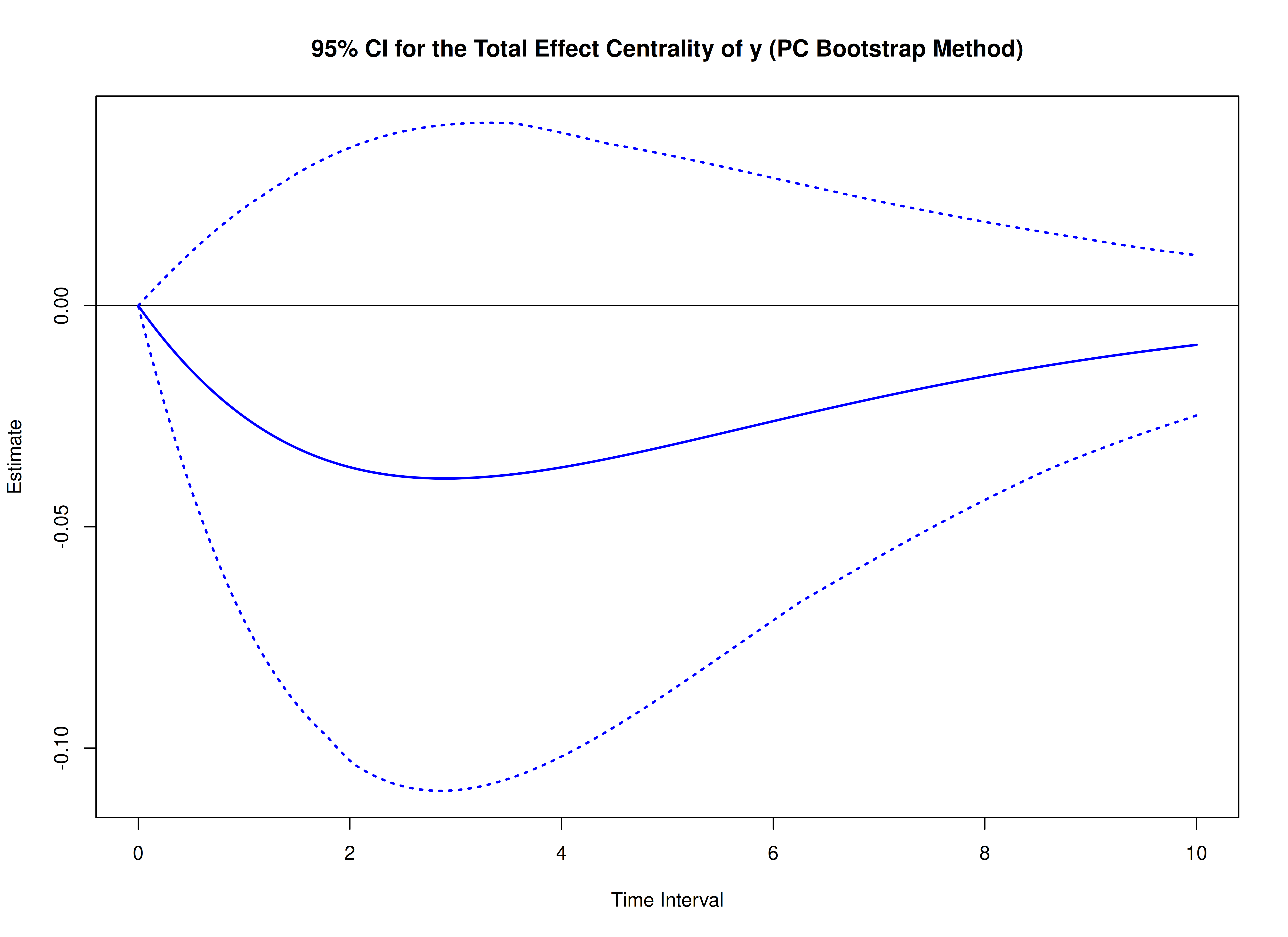
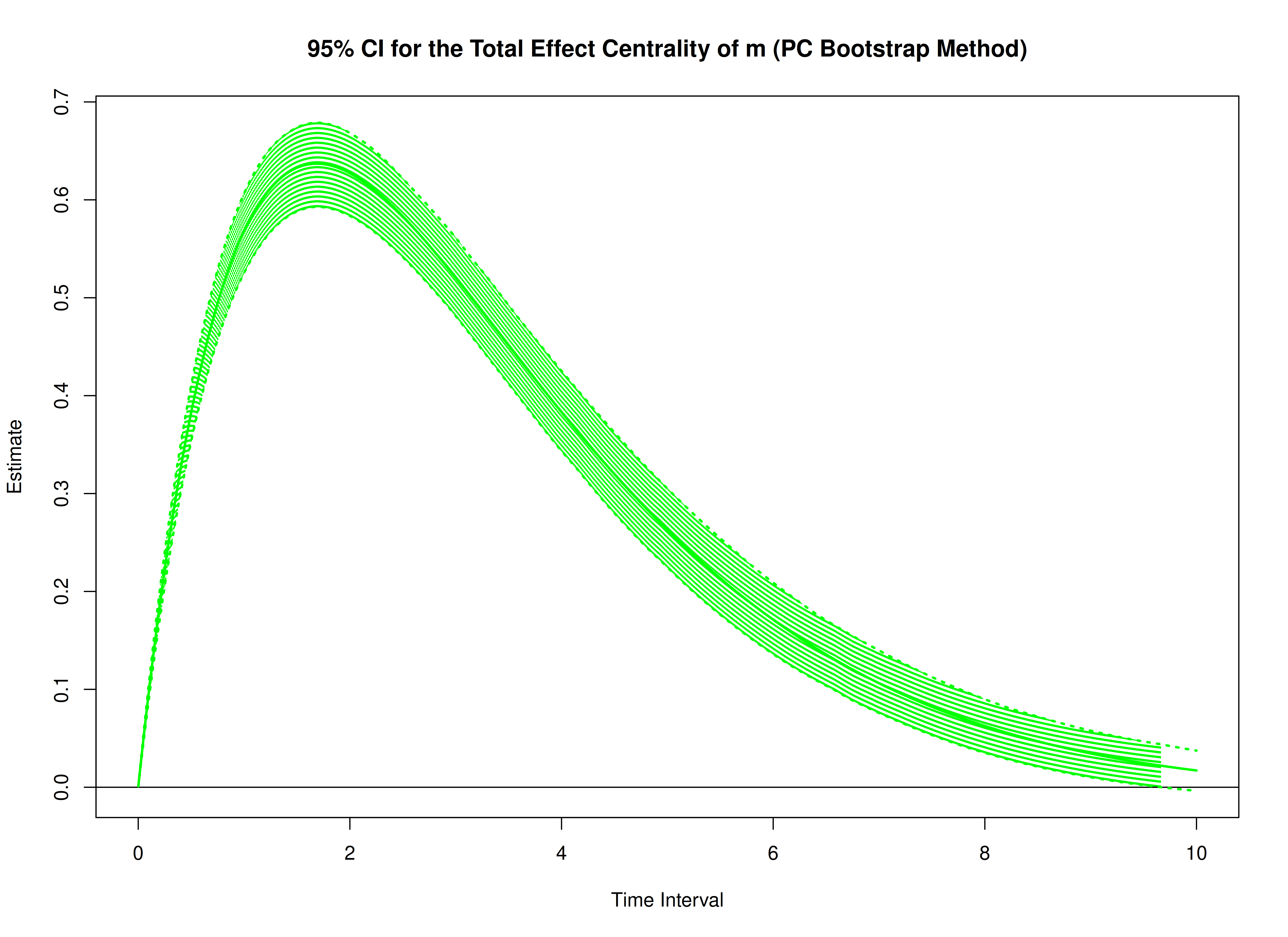
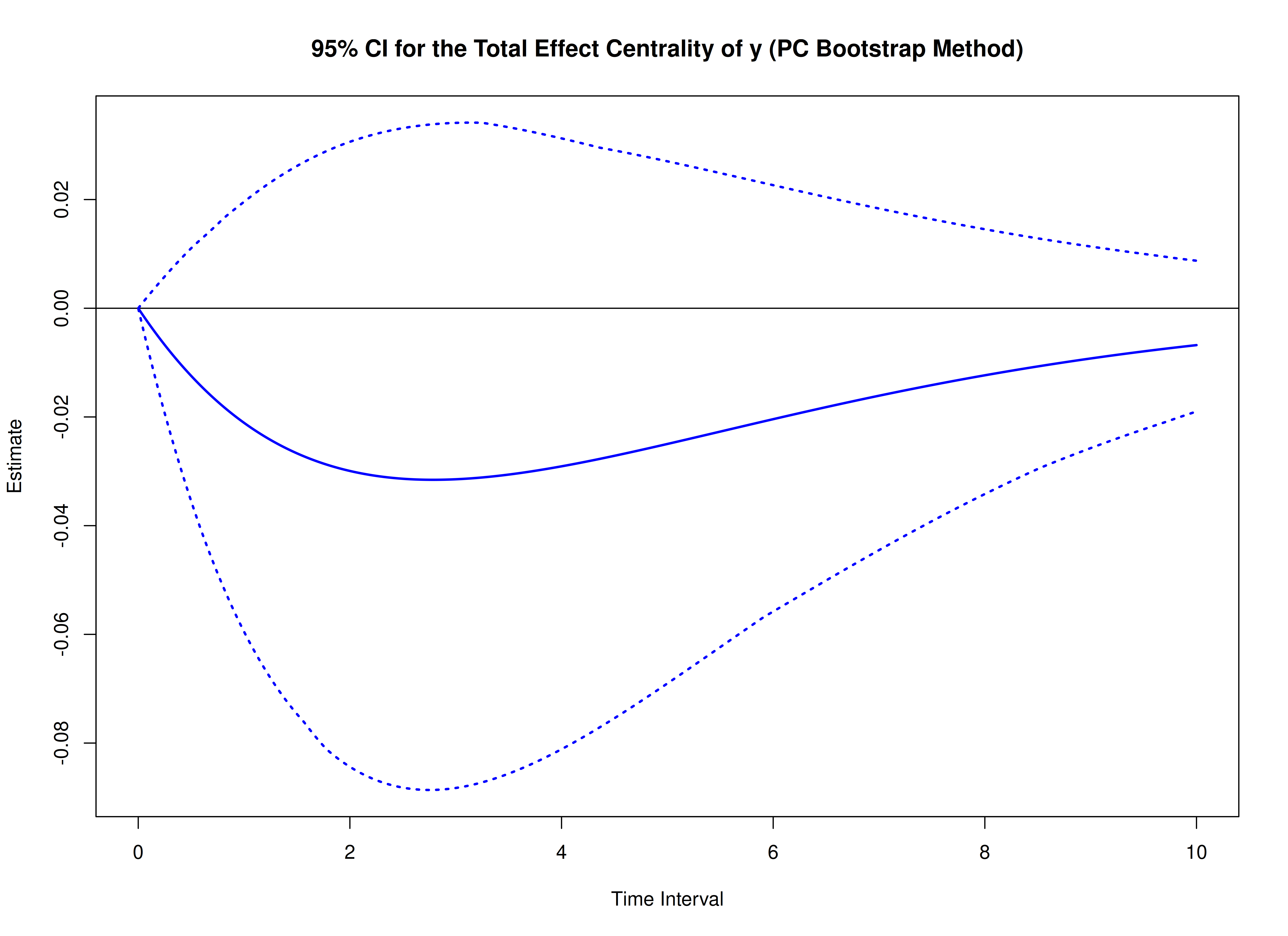
The following code generates bootstrap confidence intervals for the unstandardized total effect centrality.

library(cTMed)
boot_total <- BootTotalCentral(
  phi = phi,
  phi_hat = phi_hat,
  delta_t = delta_t,
  ncores = parallel::detectCores() # use multiple cores
)

plot(boot_total)

plot(boot_total, type = "bc")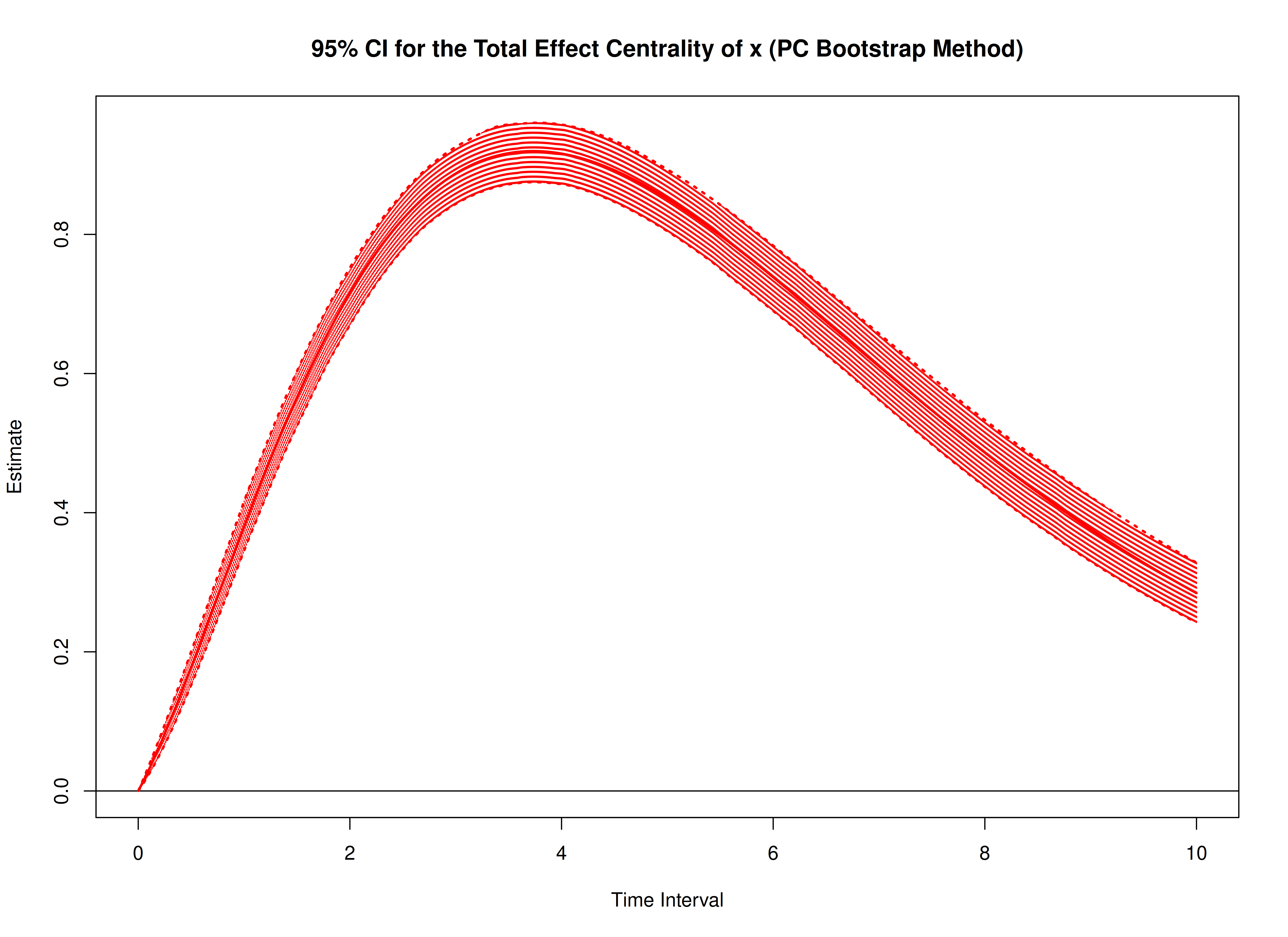

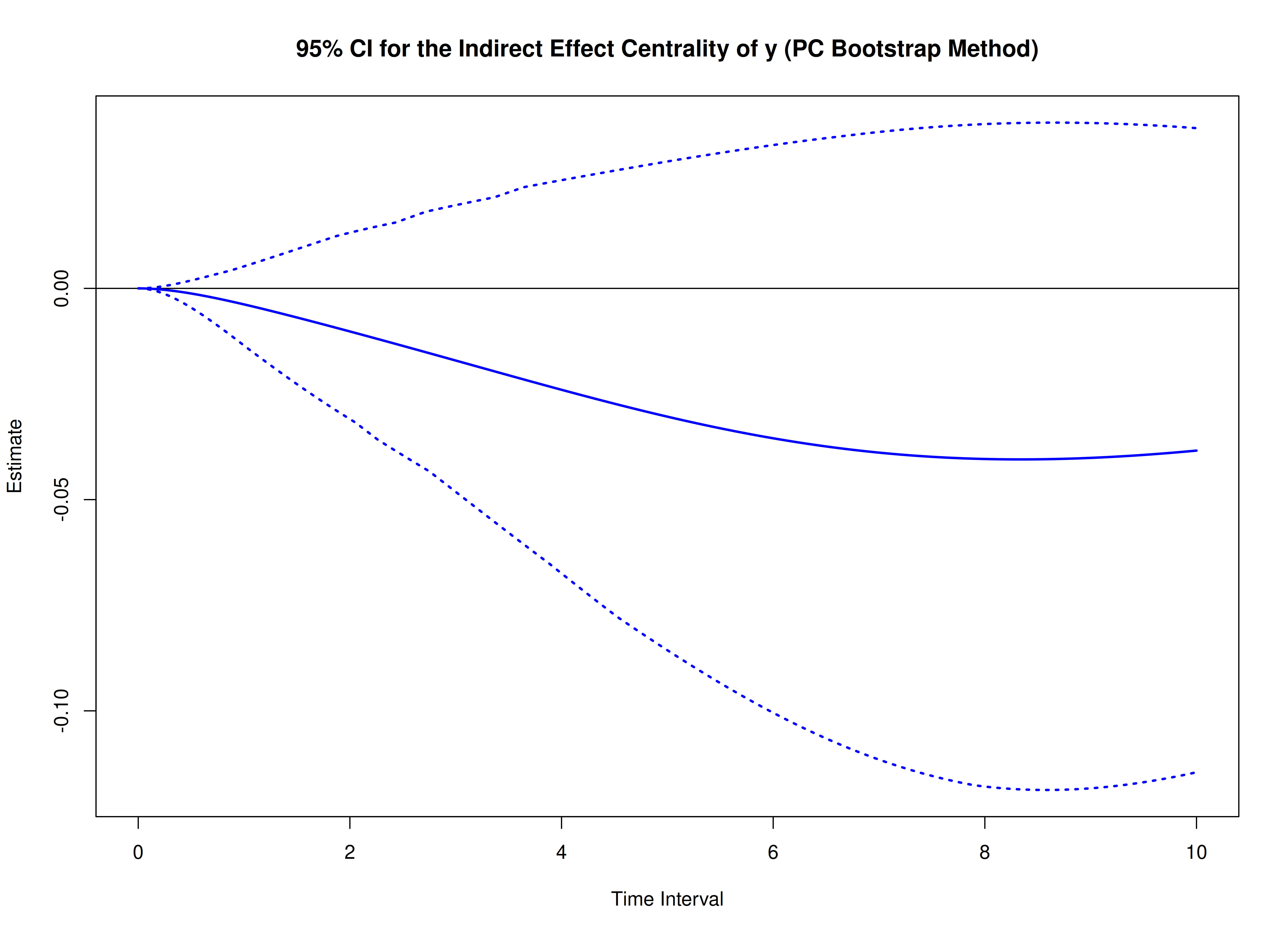
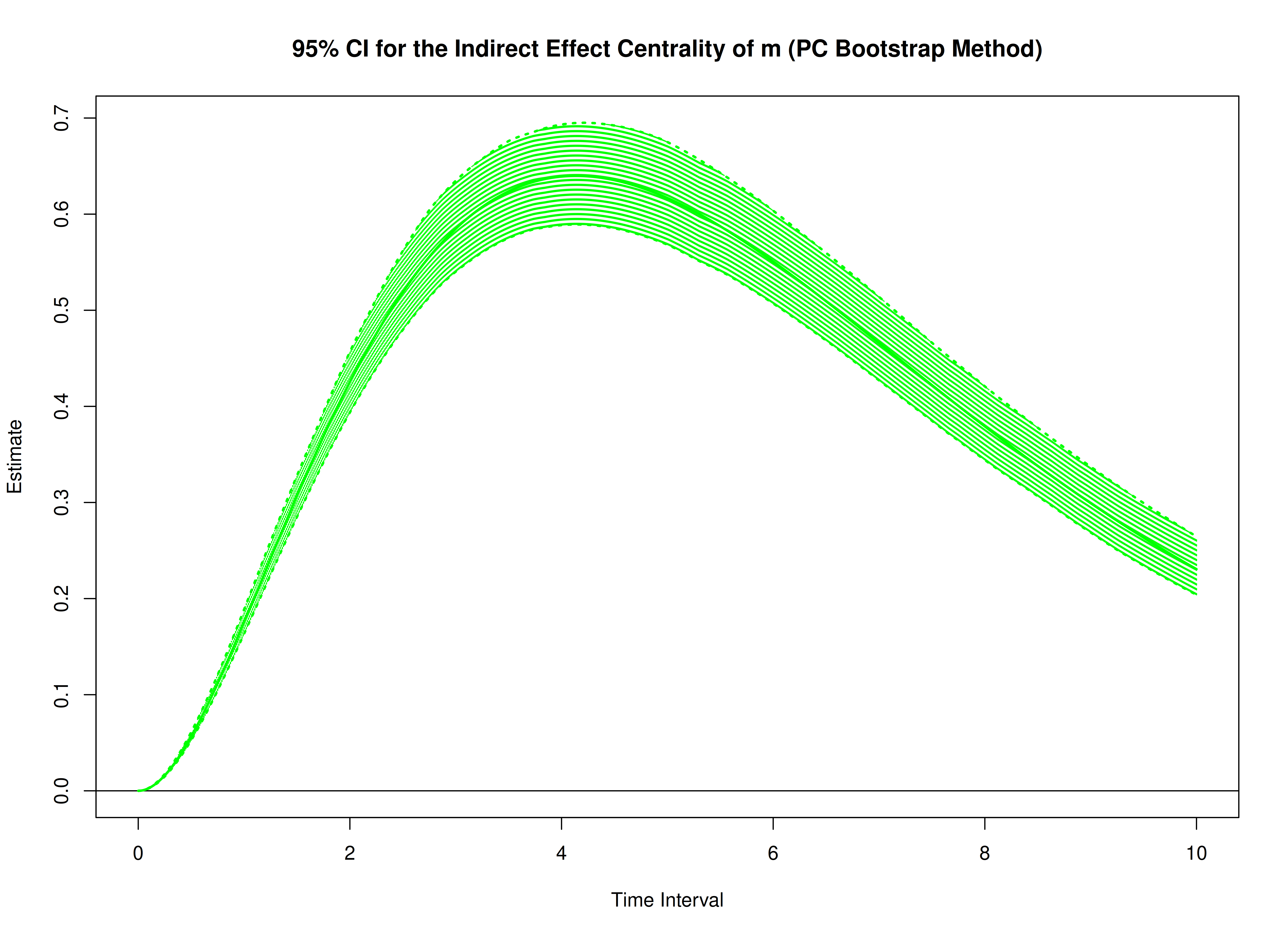
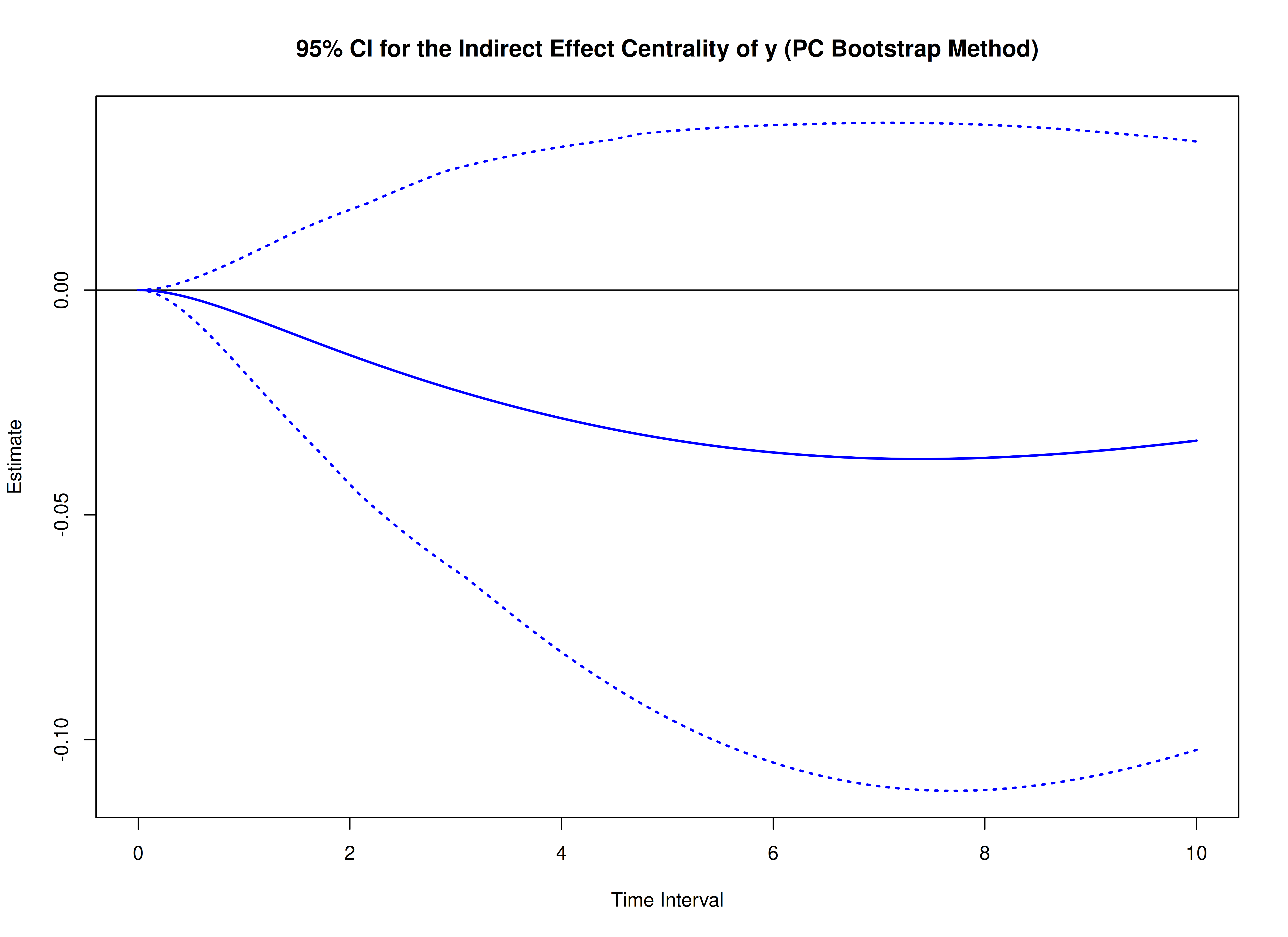
The following code generates bootstrap confidence intervals for the unstandardized indirect effect centrality.

boot_indirect <- BootIndirectCentral(
  phi = phi,
  phi_hat = phi_hat,
  delta_t = delta_t,
  ncores = parallel::detectCores() # use multiple cores
)

plot(boot_indirect)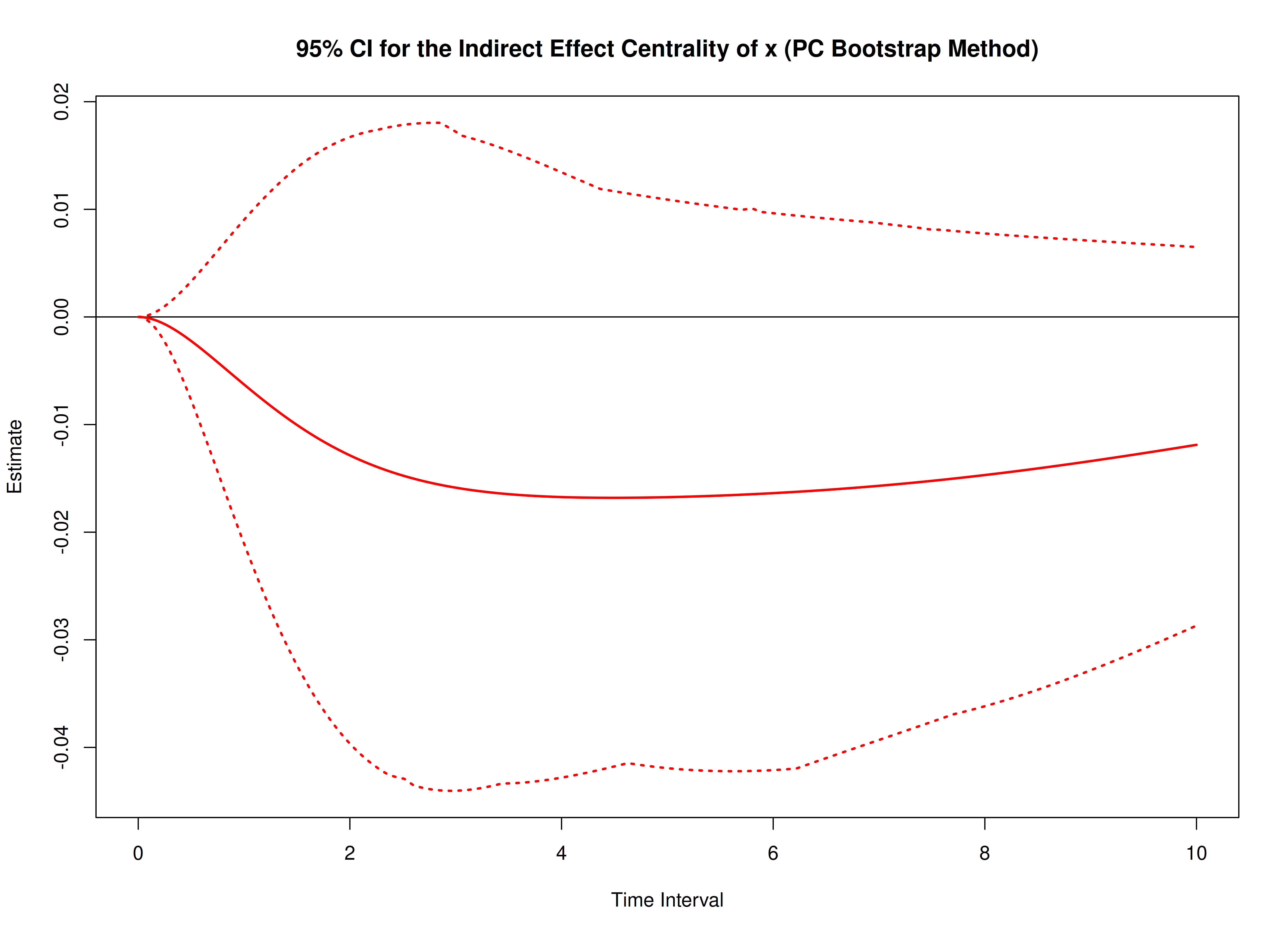

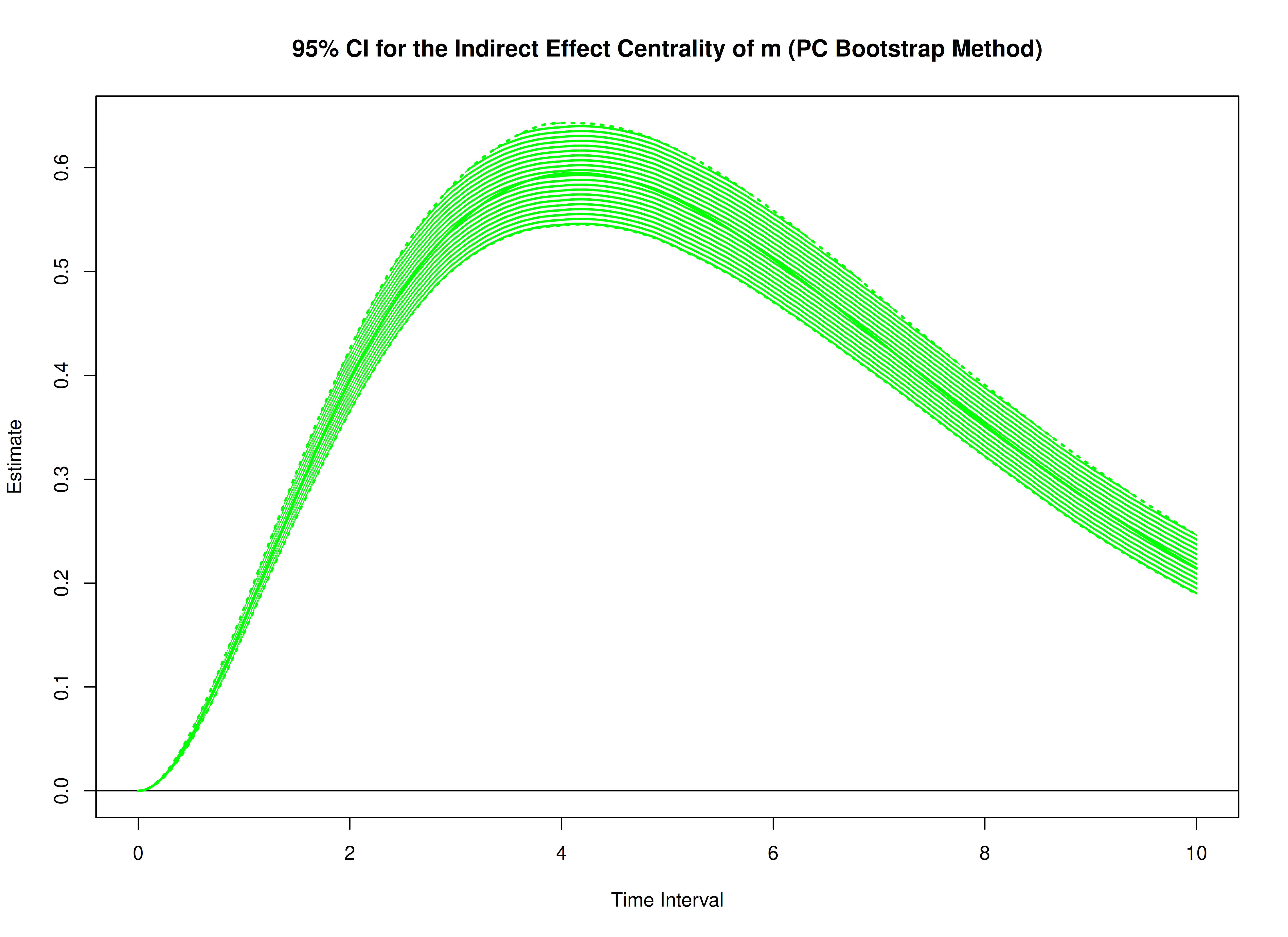
plot(boot_indirect, type = "bc")

Bootstrap Method: Standardized Centrality

The following code generates bootstrap confidence intervals for the standardized total effect centrality.

boot_total_std <- BootTotalCentralStd(
  phi = phi,
  sigma = sigma,
  phi_hat = phi_hat,
  sigma_hat = sigma_hat,
  delta_t = delta_t,
  ncores = parallel::detectCores() # use multiple cores
)

plot(boot_total_std)

plot(boot_total_std, type = "bc")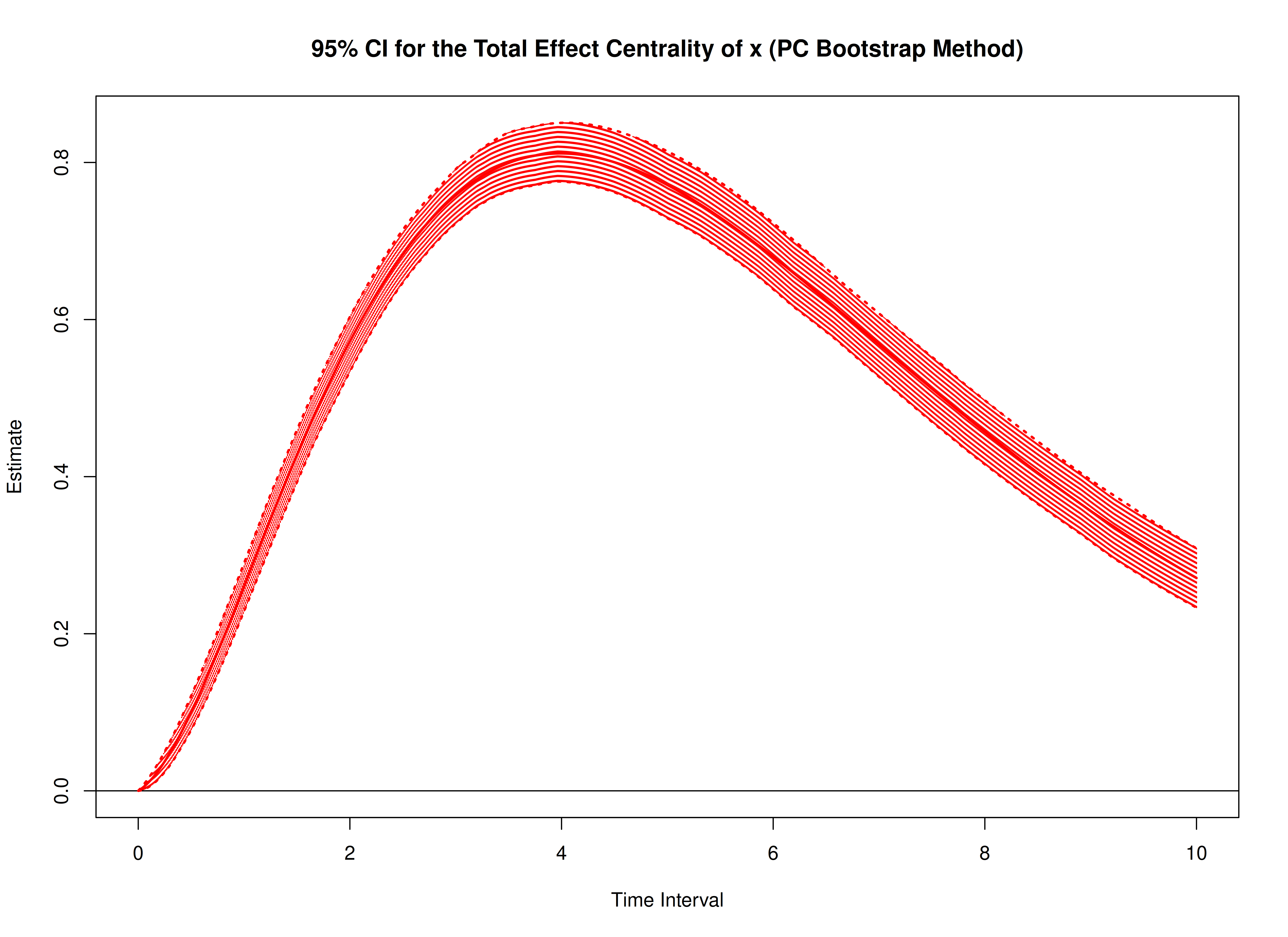

The following code generates bootstrap confidence intervals for the standardized indirect effect centrality.

boot_indirect_std <- BootIndirectCentralStd(
  phi = phi,
  sigma = sigma,
  phi_hat = phi_hat,
  sigma_hat = sigma_hat,
  delta_t = delta_t,
  ncores = parallel::detectCores() # use multiple cores
)

plot(boot_indirect_std)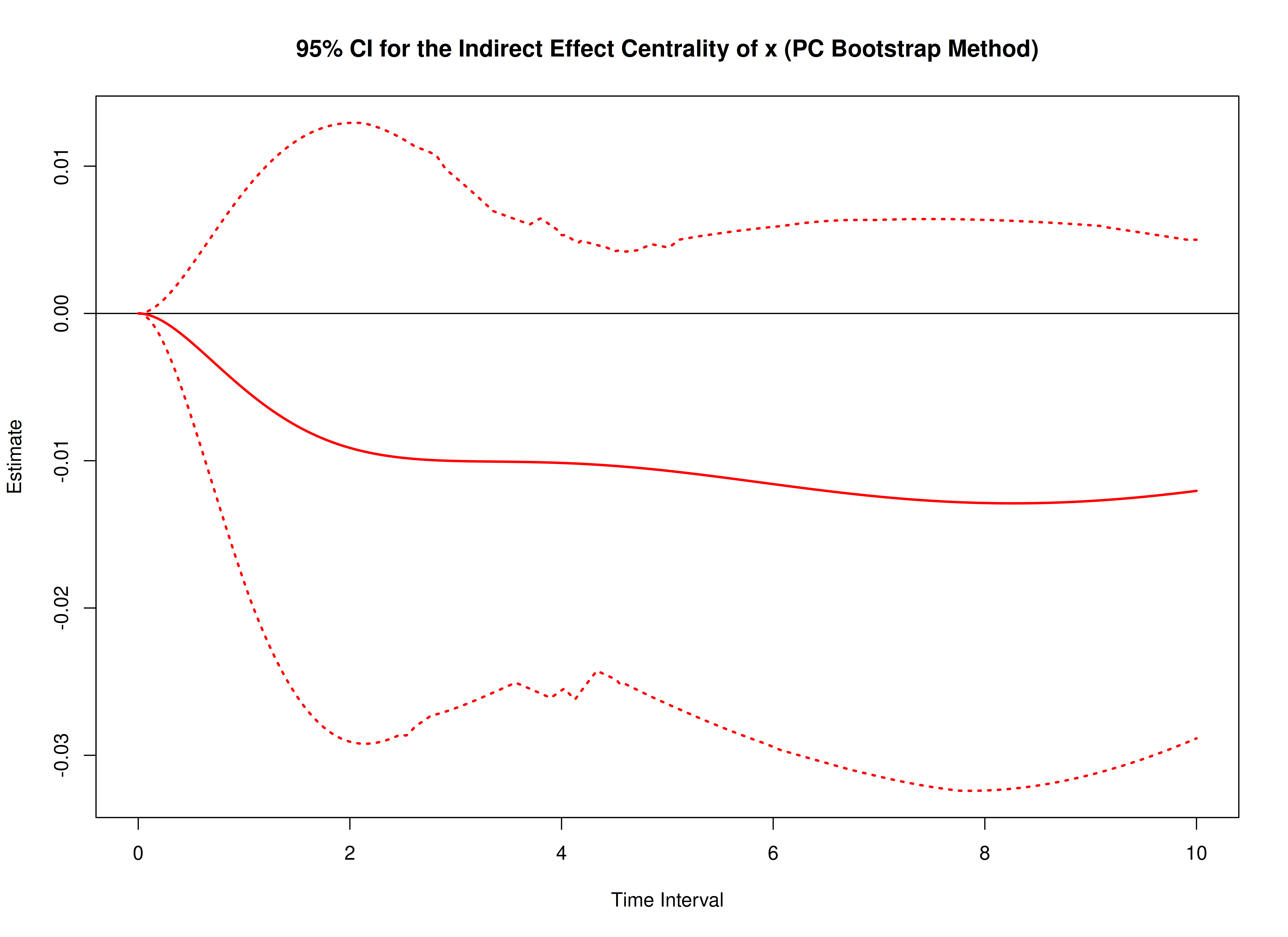

plot(boot_indirect_std, type = "bc")

References

Deboeck, P. R., & Preacher, K. J. (2015). No need to be discrete: A method for continuous time mediation analysis. Structural Equation Modeling: A Multidisciplinary Journal, 23(1), 61–75. https://doi.org/10.1080/10705511.2014.973960

Pesigan, I. J. A., Russell, M. A., & Chow, S.-M. (2025). Inferences and effect sizes for direct, indirect, and total effects in continuous-time mediation models. Psychological Methods. https://doi.org/10.1037/met0000779

R Core Team. (2026). R: A language and environment for statistical computing. R Foundation for Statistical Computing. https://www.R-project.org/

Ryan, O., & Hamaker, E. L. (2021). Time to intervene: A continuous-time approach to network analysis and centrality. Psychometrika, 87(1), 214–252. https://doi.org/10.1007/s11336-021-09767-0

Ivan Jacob Agaloos Pesigan

2026-06-15

Bootstrap Method: Unstandardized Centrality

Bootstrap Method: Standardized Centrality

References